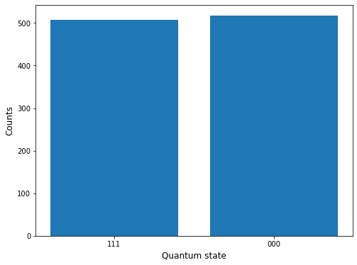
This code is an example of how you can use Python to simulate and test quantum circuits, and then plot the results of the simulation.
The code first defines a quantum circuit using a quantum register (q) and a classical register (c). The quantum circuit is constructed using the QuantumCircuit class from the Qiskit library. The circuit consists of three qubits and three classical bits, which are used to store the results of the measurements.
The code then adds gates to the quantum circuit using the h and cx functions. These gates perform operations on the qubits, such as applying a Hadamard gate (h) or a controlled-NOT gate (cx).
Next, the code measures the qubits using the measure function. This function stores the results of the measurements in the classical bits.
Finally, the code executes the quantum circuit using a quantum simulator (in this case, the qasm_simulator backend provided by Qiskit). The results of the simulation are stored in a counts dictionary, which is used to create a bar plot showing the counts for each quantum state that was observed in the simulation.
#!/usr/bin/env python3
# -*- coding: utf-8 -*-
"""
Created on Wed Dec 21 23:10:26 2022

@author: ramnot
"""

import numpy as np
import matplotlib.pyplot as plt
from qiskit import QuantumCircuit, QuantumRegister, ClassicalRegister, execute, Aer

# Define the quantum circuit
q = QuantumRegister(3)
c = ClassicalRegister(3)
qc = QuantumCircuit(q, c)

# Add gates to the circuit
qc.h(q[0])
qc.cx(q[0], q[1])
qc.cx(q[1], q[2])

# Measure the qubits
qc.measure(q, c)

# Execute the circuit using a quantum simulator
backend = Aer.get_backend('qasm_simulator')
result = execute(qc, backend, shots=1024).result()
counts = result.get_counts(qc)

# Plot the results
fig, ax = plt.subplots(figsize=(8,6))
ax.bar(counts.keys(), counts.values())
ax.set_xlabel('Quantum state', fontsize=12)
ax.set_ylabel('Counts', fontsize=12)
plt.show()


