Machine learning to optimize the design of an energy system

This code is uses machine learning in Python to optimize the design of an energy system. The energy system is defined by two variables: the energy input (in MW) and the efficiency of the system (dimensionless). The goal is to predict the cost of the energy system as a function of these variables.

To do this, the code first defines a function called cost that calculates the cost of the energy system as a function of the energy input and the efficiency. This function takes into account the cost of the energy input itself, as well as the efficiency of the system (since a more efficient system will have a lower cost).

Next, the code generates a training dataset by randomly sampling a large number of values for the energy input and efficiency. The machine learning model (a random forest regressor) is then trained on this dataset using the fit function.

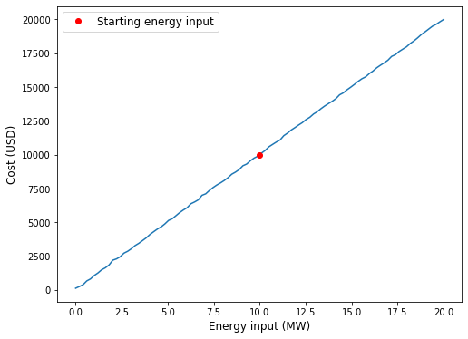
The code then generates a prediction dataset and uses the machine learning model to predict the cost for this dataset using the predict function. The resulting predictions are plotted as a function of the energy input, with the starting energy input indicated by a red dot. The resulting plot can be used to visualize how the predicted cost of the energy system changes as a function of the energy input and efficiency.

#!/usr/bin/env python3
# -*- coding: utf-8 -*-
"""
Created on Wed Dec 21 23:01:06 2022

@author: ramnot
"""

import numpy as np
import matplotlib.pyplot as plt
from sklearn.ensemble import RandomForestRegressor

# Define variables for the energy system
energy_input = 10 # MW
energy_output = 8 # MW
efficiency = energy_output / energy_input # dimensionless

# Define the cost function
def cost(energy_input, efficiency):
  # Assume a cost of $1000/MW for energy input
  return energy_input * 1000 + efficiency**2

# Generate a training dataset
num_samples = 1000
X_train = np.random.uniform(0, 20, (num_samples, 2))
y_train = cost(X_train[:,0], X_train[:,1])

# Use machine learning to predict the cost as a function of the energy input and efficiency
model = RandomForestRegressor()
model.fit(X_train, y_train)

# Generate a prediction dataset
energy_input_range = np.linspace(0, 20, 100)
X_pred = np.column_stack((energy_input_range, np.ones_like(energy_input_range)*efficiency))

# Use the machine learning model to predict the cost for the prediction dataset
y_pred = model.predict(X_pred)

# Plot the predicted cost as a function of the energy input
fig, ax = plt.subplots(figsize=(8,6))
ax.plot(energy_input_range, y_pred)
ax.plot(energy_input, cost(energy_input, efficiency), 'o', color='red', label='Starting energy input')
ax.set_xlabel('Energy input (MW)', fontsize=12)
ax.set_ylabel('Cost (USD)', fontsize=12)
ax.legend(fontsize=12)
plt.show()

Optimize the design of an energy system

This code is an example of how you could use Python to optimize the design of an energy system. The energy system is defined by two variables: the energy input (in MW) and the efficiency of the system (dimensionless). The goal is to find the optimal value of the energy input that will result in the lowest cost for the system.

To do this, the code defines a function called cost that calculates the cost of the energy system as a function of the energy input and the efficiency. This function takes into account the cost of the energy input itself, as well as the efficiency of the system (since a more efficient system will have a lower cost).

Then, the code uses an optimization algorithm to find the optimal value of the energy input that minimizes the cost function. The optimization algorithm is given the starting value of the energy input, and it iteratively adjusts this value to find the minimum of the cost function.

Finally, the code generates a grid of possible energy input values and calculates the cost at each point on the grid. It then plots the cost as a function of the energy input, with the starting energy input indicated by a red dot and the optimal energy input indicated by a blue dot. The resulting plot can be used to visualize how the cost of the energy system changes as a function of the energy input, and to see how the optimal energy input compares to the starting energy input.

#!/usr/bin/env python3
# -*- coding: utf-8 -*-
"""
Created on Wed Dec 21 22:53:22 2022

@author: ramnot
"""

import numpy as np
import scipy.optimize as optimize
import matplotlib.pyplot as plt

# Define variables for the energy system
energy_input = 10 # MW
energy_output = 8 # MW
efficiency = energy_output / energy_input # dimensionless

# Define the cost function
def cost(energy_input, efficiency):
  # Assume a cost of $1000/MW for energy input
  return energy_input * 1000 + efficiency**2

# Use optimization algorithm to find the optimal energy input
result = optimize.minimize(cost, energy_input, args=(efficiency,), method='nelder-mead')
optimal_energy_input = result.x

# Generate a grid of energy input values
energy_input_range = np.linspace(0, 20, 100)

# Calculate the cost at each point on the grid
cost_values = np.zeros_like(energy_input_range)
for i in range(energy_input_range.shape[0]):
  cost_values[i] = cost(energy_input_range[i], efficiency)

# Plot the cost as a function of the energy input
fig, ax = plt.subplots(figsize=(8,6))
ax.plot(energy_input_range, cost_values)
ax.plot(energy_input, cost(energy_input, efficiency), 'o', color='red', label='Starting energy input')
ax.plot(optimal_energy_input, cost(optimal_energy_input, efficiency), 'o', color='blue', label='Optimal energy input')
ax.set_xlabel('Energy input (MW)', fontsize=12)
ax.set_ylabel('Cost (USD)', fontsize=12)
ax.legend(fontsize=12)
plt.show()