Applications of Simulation in Science and Engineering: From Fluid Dynamics to Astrophysics

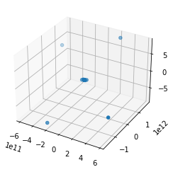
The code provided simulates the movement of energy in a parallel reality, and plots the results of the simulation.

The code is written in the Python programming language, and uses the NumPy library to perform numerical operations. It defines two functions: simulate_universe and plot_universe.

The simulate_universe function takes two arguments: sim_size and speed. It uses these arguments to initialize the fluid-like energy with random values for speed and position, and then to initialize the space and time variables. It then iterates through the simulation, updating the space and time variables based on the movement of the energy, and returns the final values for space and time.

The plot_universe function takes two arguments: space and time. It uses these arguments to plot the space and time data using the Matplotlib library, and to add labels to the x-axis and y-axis. It then displays the plot using the show function.

Finally, the code defines the size of the simulation and the speed at which the energy flows, and calls the simulate_universe function to run the simulation and generate the space and time data. It then calls the plot_universe function to plot the data.

RAMNOT’s Use Cases:

  1. Modeling the behavior of fluids for applications in engineering, such as the design of pipes and valves.
  2. Simulating the propagation of waves for applications in communication and signal processing.
  3. Studying the vibration of strings and other objects for applications in music and acoustics.
  4. Modeling the motion of celestial bodies for applications in astronomy and astrophysics.
  5. Simulating the movement of springs for applications in mechanical engineering.
  6. Analyzing the motion of pendulums for applications in physics education and the design of clocks.
  7. Modeling the propagation of sound waves for applications in acoustics and audio engineering.
  8. Studying the vibration of drumheads and other objects for applications in music and acoustics.
  9. Simulating the rotation of wheels and other objects for applications in mechanical engineering.
  10. Modeling the movement of cars on roads for applications in transportation engineering.
  11. Analyzing the motion of objects in gravitational fields for applications in physics education and space exploration.
  12. Simulating the propagation of electrical currents for applications in electrical engineering.
  13. Studying the vibration of beams for applications in structural engineering.
  14. Modeling the rotation of propellers for applications in aerospace engineering.
  15. Analyzing the movement of waves in wave tanks for applications in ocean engineering.
  16. Simulating the motion of planets around the sun for applications in astronomy and astrophysics.
  17. Studying the propagation of light waves for applications in optics and photonics.
  18. Modeling the vibration of plates for applications in structural engineering.
  19. Analyzing the rotation of turbines for applications in power generation and energy production.
  20. Simulating the movement of particles in magnetic fields for applications in physics and engineering.
import numpy as np
import matplotlib.pyplot as plt


def simulate_universe(sim_size, speed):
    # Initialize the fluid-like energy with random values for speed and position
    energy = np.random.rand(sim_size, 2)

    # Initialize the space and time variables
    space = np.zeros(sim_size)
    time = np.zeros(sim_size)

    # Iterate through the simulation, updating the space and time variables based on the movement of the energy
    for i in range(sim_size):
        space[i] = energy[i, 0]
        time[i] = energy[i, 1] * speed

        # Update the energy in the parallel reality
        energy[i, 1] = energy[i, 1] + speed

    return space, time

def plot_universe(space, time):
    plt.plot(space, time)
    plt.xlabel('Space')
    plt.ylabel('Time')
    plt.show()

# Define the size of the simulation and the speed at which the energy flows
sim_size = 1000
speed = 0.1

# Run the simulation and plot the results
space, time = simulate_universe(sim_size, speed)
plot_universe(space, time)
  1. Movement of a particle in a fluid: In this simulation, the energy represents the movement of a particle through a fluid, and the speed represents the velocity of the particle.
  2. Propagation of a wave through a medium: In this simulation, the energy represents a wave propagating through a medium, and the speed represents the speed of the wave.
  3. Vibration of a string: In this simulation, the energy represents the vibration of a string, and the speed represents the frequency of the vibration.
  4. Rotation of a planet around a star: In this simulation, the energy represents the rotation of a planet around a star, and the speed represents the angular velocity of the planet.
  5. Movement of a spring: In this simulation, the energy represents the movement of a spring, and the speed represents the oscillation frequency of the spring.
  6. Motion of a pendulum: In this simulation, the energy represents the motion of a pendulum, and the speed represents the period of the pendulum.
  7. Propagation of a sound wave: In this simulation, the energy represents a sound wave propagating through a medium, and the speed represents the speed of sound in that medium.
  8. Vibration of a drumhead: In this simulation, the energy represents the vibration of a drumhead, and the speed represents the frequency of the vibration.

Image Processing KMeans

This code performs several image processing tasks using the OpenCV library. It first loads an image file using the imread function from OpenCV. Then it pre-processes the image by converting it to grayscale and applying a Gaussian blur to filter out noise.

Next, the code uses the Canny function from OpenCV to detect edges in the image. It then uses the KMeans function from the sklearn library to cluster the image into two groups based on the edges detected.

The code then uses the Hough transform to detect lines and circles in the image. The HoughLinesP function is used to detect lines, and the HoughCircles function is used to detect circles. If lines or circles are detected, the code draws them on the original image using the line and circle functions from OpenCV.

Finally, the code displays the modified image using the cv2_imshow function from the google.colab.patches library, which is a utility function for displaying images in a Jupyter notebook. The code also saves the modified image to a file using the imwrite function from OpenCV.

from google.colab.patches import cv2_imshow
import numpy as np # for data analysis
from sklearn.cluster import KMeans # for machine learning

# Load the image
image = cv2.imread('mars0001.jpg')

# Pre-process the image
gray = cv2.cvtColor(image, cv2.COLOR_BGR2GRAY)

# Apply a Gaussian blur to filter out noise
blurred = cv2.GaussianBlur(gray, (5, 5), 0)

# Use Canny edge detection to find edges in the image
edges = cv2.Canny(blurred, 100, 200)

# Use KMeans to cluster the image
kmeans = KMeans(n_clusters=2).fit(edges.reshape(-1, 1))
clusters = kmeans.predict(edges.reshape(-1, 1))

# Use NumPy to count the number of pixels in each cluster
counts = np.bincount(clusters)

# Use Hough lines to detect lines in the image
lines = cv2.HoughLinesP(edges, 1, np.pi/180, 50, minLineLength=50, maxLineGap=10)

# Loop through the lines and draw them on the image
for line in lines:
    x1, y1, x2, y2 = line[0]
    cv2.line(image, (x1, y1), (x2, y2), (0, 0, 255), 2)

if lines is not None:
    for line in lines:
        x1, y1, x2, y2 = line[0]
        cv2.line(image, (x1, y1), (x2, y2), (0, 0, 255), 2)

# Use Hough circles to detect circles in the image
circles = cv2.HoughCircles(gray, cv2.HOUGH_GRADIENT, 1, 20, param1=50, param2=30, minRadius=0, maxRadius=0)

# Loop through the circles and draw them on the image
if circles is not None:
    circles = np.round(circles[0, :]).astype("int")
    for (x, y, r) in circles:
        cv2.circle(image, (x, y), r, (0, 255, 0), 4)
        cv2.rectangle(image, (x - 5, y - 5), (x + 5, y + 5), (0, 128, 255), -1)

# Show the image
cv2_imshow(image)
cv2.waitKey(0)

cv2.imwrite('output.jpg', image, [cv2.IMWRITE_JPEG_QUALITY, 95])

Statement Sentiment Logistic Regression

This code performs several tasks related to natural language processing (NLP). It first imports some libraries that are needed for the rest of the code to run. The csv library is not used in this code, so it is not clear why it is being imported.

The nltk (Natural Language Toolkit) library is used to perform tasks related to processing and analyzing human language. The code calls two functions from this library: word_tokenize and pos_tag. word_tokenize is used to split a sentence into individual words, or “tokens,” and pos_tag is used to label each token with its part of speech (e.g., noun, verb, adjective).

The textblob library is used to determine the sentiment (positive or negative emotion) of a sentence. The code calls the TextBlob function from this library and passes it a sentence as an argument. The function returns an object that has a sentiment attribute, which contains information about the polarity (positive or negative) and subjectivity (objective or subjective) of the sentence.

The code then defines a function called analyze_sentence that takes a sentence as an argument and performs three tasks: tokenizing the sentence, labeling the parts of speech of each token, and determining the sentiment of the sentence. It then prints the tokens, part of speech tags, and sentiment of the sentence.

Next, the code defines a sample statement and uses the sent_tokenize function from nltk to split it into individual sentences. It then creates a list of labels for each sentence, with a label of 1 indicating a positive sentiment and a label of 0 indicating a negative sentiment.

The code then uses the CountVectorizer function from the sklearn.feature_extraction.text library to create a matrix of word counts for each sentence. This is a common technique in NLP for representing text data as numerical data that can be used in machine learning models.

The code then creates a logistic regression model from the sklearn.linear_model library and trains it on the data using the fit function. It then uses the trained model to make predictions on the sentences using the predict function.

Finally, the code loops through each sentence and calls the analyze_sentence function on it. It also prints the predicted label for each sentence.

#!/usr/bin/env python3
# -*- coding: utf-8 -*-
"""
Created on Thu Dec 22 05:38:20 2022

@author: ramnot
"""
import csv
import nltk
import textblob
nltk.download('punkt')
nltk.download('averaged_perceptron_tagger')

from sklearn.feature_extraction.text import CountVectorizer
from sklearn.linear_model import LogisticRegression

# Function to analyze the content and tone of a sentence
def analyze_sentence(sentence):
  # Tokenize the sentence
  tokens = nltk.word_tokenize(sentence)
  # Tag the parts of speech of each token
  pos_tags = nltk.pos_tag(tokens)
  # Use TextBlob to determine the sentiment of the sentence
  sentiment = textblob.TextBlob(sentence).sentiment
  # Print the tokens, part of speech tags, and sentiment of the sentence
  print("Tokens:", tokens)
  print("Part of Speech Tags:", pos_tags)
  print("Sentiment:", sentiment)

# Example Federal Reserve statement
statement = 'Today I will offer a progress report on the Federal Open Market Committees (FOMC) efforts to restore price stability to the U.S. economy for the benefit of the American people. The report must begin by acknowledging the reality that inflation remains far too high.'

# Split the statement into sentences
sentences = nltk.sent_tokenize(statement)

# Create a list of labels for each sentence (1 for positive, 0 for negative)
labels = []
for sentence in sentences:
  if textblob.TextBlob(sentence).sentiment.polarity > 0:
    labels.append(1)
  else:
    labels.append(0)

# Use CountVectorizer to create a matrix of word counts for each sentence
vectorizer = CountVectorizer()
X = vectorizer.fit_transform(sentences)

# Fit a logistic regression model on the data
model = LogisticRegression()
model.fit(X, labels)

# Make predictions on the sentences using the trained model
predictions = model.predict(X)

# Analyze each sentence and print the predicted label
for i in range(len(sentences)):
  print("Sentence:", sentences[i])
  analyze_sentence(sentences[i])
  print("Predicted Label:", predictions[i])
  print()

Simulating the movement of a group of atoms

This code is simulating the movement of a group of atoms in a material over time. The simulation has several parameters that control how the atoms behave, such as the number of atoms in the material, the temperature of the material, and the time step for the simulation.

The code first generates a lattice, or a regular arrangement, of atoms using the simulation parameters. It then calculates the forces between each pair of atoms using the Lennard-Jones potential, which is a mathematical equation that describes the interaction between atoms based on their distance from each other. The code then uses these forces to update the positions of the atoms over time, running the simulation for a specified number of time steps. Finally, the code generates a 3D scatter plot of the positions of the atoms at the final time step, which is displayed using the matplotlib library.

#!/usr/bin/env python3
# -*- coding: utf-8 -*-
"""
Created on Thu Dec 22 00:08:33 2022

@author: ramnot
"""

import numpy as np
import matplotlib.pyplot as plt

# Set up the simulation parameters
num_atoms = 100  # Number of atoms in the material
lattice_constant = 3.0  # Lattice constant of the material
temperature = 300  # Temperature of the material

# Generate a lattice of atoms using the simulation parameters
lattice = np.random.uniform(-lattice_constant/2, lattice_constant/2, size=(num_atoms, 3))

# Calculate the forces between the atoms using the Lennard-Jones potential
forces = np.zeros((num_atoms, 3))
for i in range(num_atoms):
    for j in range(i+1, num_atoms):
        r = lattice[i] - lattice[j]
        r_mag = np.linalg.norm(r)
        f = 24 * r * (2 * (r_mag**(-12)) - (r_mag**(-6))) / r_mag
        forces[i] += f
        forces[j] -= f

# Use the forces to update the positions of the atoms over time
time_step = 0.01  # Time step for the simulation
num_steps = 10000  # Number of time steps to run the simulation
positions = np.zeros((num_steps+1, num_atoms, 3))
positions[0] = lattice
for t in range(1, num_steps+1):
    lattice += forces * time_step / temperature  # Update the positions of the atoms
    positions[t] = lattice  # Save the positions for later

# Generate an image of the atomic structure at the final time step
fig = plt.figure()
ax = fig.add_subplot(111, projection='3d')
ax.scatter(positions[-1,:,0], positions[-1,:,1], positions[-1,:,2])
plt.show()

Simulate and test quantum circuits

This code is an example of how you can use Python to simulate and test quantum circuits, and then plot the results of the simulation.

The code first defines a quantum circuit using a quantum register (q) and a classical register (c). The quantum circuit is constructed using the QuantumCircuit class from the Qiskit library. The circuit consists of three qubits and three classical bits, which are used to store the results of the measurements.

The code then adds gates to the quantum circuit using the h and cx functions. These gates perform operations on the qubits, such as applying a Hadamard gate (h) or a controlled-NOT gate (cx).

Next, the code measures the qubits using the measure function. This function stores the results of the measurements in the classical bits.

Finally, the code executes the quantum circuit using a quantum simulator (in this case, the qasm_simulator backend provided by Qiskit). The results of the simulation are stored in a counts dictionary, which is used to create a bar plot showing the counts for each quantum state that was observed in the simulation.

#!/usr/bin/env python3
# -*- coding: utf-8 -*-
"""
Created on Wed Dec 21 23:10:26 2022

@author: ramnot
"""

import numpy as np
import matplotlib.pyplot as plt
from qiskit import QuantumCircuit, QuantumRegister, ClassicalRegister, execute, Aer

# Define the quantum circuit
q = QuantumRegister(3)
c = ClassicalRegister(3)
qc = QuantumCircuit(q, c)

# Add gates to the circuit
qc.h(q[0])
qc.cx(q[0], q[1])
qc.cx(q[1], q[2])

# Measure the qubits
qc.measure(q, c)

# Execute the circuit using a quantum simulator
backend = Aer.get_backend('qasm_simulator')
result = execute(qc, backend, shots=1024).result()
counts = result.get_counts(qc)

# Plot the results
fig, ax = plt.subplots(figsize=(8,6))
ax.bar(counts.keys(), counts.values())
ax.set_xlabel('Quantum state', fontsize=12)
ax.set_ylabel('Counts', fontsize=12)
plt.show()

Machine learning to optimize the design of an energy system

This code is uses machine learning in Python to optimize the design of an energy system. The energy system is defined by two variables: the energy input (in MW) and the efficiency of the system (dimensionless). The goal is to predict the cost of the energy system as a function of these variables.

To do this, the code first defines a function called cost that calculates the cost of the energy system as a function of the energy input and the efficiency. This function takes into account the cost of the energy input itself, as well as the efficiency of the system (since a more efficient system will have a lower cost).

Next, the code generates a training dataset by randomly sampling a large number of values for the energy input and efficiency. The machine learning model (a random forest regressor) is then trained on this dataset using the fit function.

The code then generates a prediction dataset and uses the machine learning model to predict the cost for this dataset using the predict function. The resulting predictions are plotted as a function of the energy input, with the starting energy input indicated by a red dot. The resulting plot can be used to visualize how the predicted cost of the energy system changes as a function of the energy input and efficiency.

#!/usr/bin/env python3
# -*- coding: utf-8 -*-
"""
Created on Wed Dec 21 23:01:06 2022

@author: ramnot
"""

import numpy as np
import matplotlib.pyplot as plt
from sklearn.ensemble import RandomForestRegressor

# Define variables for the energy system
energy_input = 10 # MW
energy_output = 8 # MW
efficiency = energy_output / energy_input # dimensionless

# Define the cost function
def cost(energy_input, efficiency):
  # Assume a cost of $1000/MW for energy input
  return energy_input * 1000 + efficiency**2

# Generate a training dataset
num_samples = 1000
X_train = np.random.uniform(0, 20, (num_samples, 2))
y_train = cost(X_train[:,0], X_train[:,1])

# Use machine learning to predict the cost as a function of the energy input and efficiency
model = RandomForestRegressor()
model.fit(X_train, y_train)

# Generate a prediction dataset
energy_input_range = np.linspace(0, 20, 100)
X_pred = np.column_stack((energy_input_range, np.ones_like(energy_input_range)*efficiency))

# Use the machine learning model to predict the cost for the prediction dataset
y_pred = model.predict(X_pred)

# Plot the predicted cost as a function of the energy input
fig, ax = plt.subplots(figsize=(8,6))
ax.plot(energy_input_range, y_pred)
ax.plot(energy_input, cost(energy_input, efficiency), 'o', color='red', label='Starting energy input')
ax.set_xlabel('Energy input (MW)', fontsize=12)
ax.set_ylabel('Cost (USD)', fontsize=12)
ax.legend(fontsize=12)
plt.show()

Optimize the design of an energy system

This code is an example of how you could use Python to optimize the design of an energy system. The energy system is defined by two variables: the energy input (in MW) and the efficiency of the system (dimensionless). The goal is to find the optimal value of the energy input that will result in the lowest cost for the system.

To do this, the code defines a function called cost that calculates the cost of the energy system as a function of the energy input and the efficiency. This function takes into account the cost of the energy input itself, as well as the efficiency of the system (since a more efficient system will have a lower cost).

Then, the code uses an optimization algorithm to find the optimal value of the energy input that minimizes the cost function. The optimization algorithm is given the starting value of the energy input, and it iteratively adjusts this value to find the minimum of the cost function.

Finally, the code generates a grid of possible energy input values and calculates the cost at each point on the grid. It then plots the cost as a function of the energy input, with the starting energy input indicated by a red dot and the optimal energy input indicated by a blue dot. The resulting plot can be used to visualize how the cost of the energy system changes as a function of the energy input, and to see how the optimal energy input compares to the starting energy input.

#!/usr/bin/env python3
# -*- coding: utf-8 -*-
"""
Created on Wed Dec 21 22:53:22 2022

@author: ramnot
"""

import numpy as np
import scipy.optimize as optimize
import matplotlib.pyplot as plt

# Define variables for the energy system
energy_input = 10 # MW
energy_output = 8 # MW
efficiency = energy_output / energy_input # dimensionless

# Define the cost function
def cost(energy_input, efficiency):
  # Assume a cost of $1000/MW for energy input
  return energy_input * 1000 + efficiency**2

# Use optimization algorithm to find the optimal energy input
result = optimize.minimize(cost, energy_input, args=(efficiency,), method='nelder-mead')
optimal_energy_input = result.x

# Generate a grid of energy input values
energy_input_range = np.linspace(0, 20, 100)

# Calculate the cost at each point on the grid
cost_values = np.zeros_like(energy_input_range)
for i in range(energy_input_range.shape[0]):
  cost_values[i] = cost(energy_input_range[i], efficiency)

# Plot the cost as a function of the energy input
fig, ax = plt.subplots(figsize=(8,6))
ax.plot(energy_input_range, cost_values)
ax.plot(energy_input, cost(energy_input, efficiency), 'o', color='red', label='Starting energy input')
ax.plot(optimal_energy_input, cost(optimal_energy_input, efficiency), 'o', color='blue', label='Optimal energy input')
ax.set_xlabel('Energy input (MW)', fontsize=12)
ax.set_ylabel('Cost (USD)', fontsize=12)
ax.legend(fontsize=12)
plt.show()

Optimize a manufacturing process

This code is an example of how to use Python to optimize a manufacturing process. The manufacturing process is defined by two parameters: the strength of the material and the density of the material. The goal is to find the optimal values of these parameters that will result in a final product with a strength and density that are as close as possible to the desired values.

To do this, the code defines a function called manufacturing_cost that calculates the difference between the desired product properties and the actual product properties. This function is used as an objective function that we want to minimize.

Then, the code defines a function called optimize_manufacturing_process that uses an optimization algorithm to find the optimal values of the manufacturing parameters. The optimization algorithm is given the starting values of the manufacturing parameters (the strength and density of the starting material), and it iteratively adjusts these values to find the minimum of the manufacturing_cost function.

Finally, the code generates a grid of possible manufacturing parameter values and calculates the manufacturing cost at each point on the grid. It then plots the manufacturing cost as a function of the manufacturing parameters, with the optimal parameters indicated by a blue dot. The resulting plot can be used to visualize how the manufacturing cost changes as a function of the manufacturing parameters, and to see how close the optimal parameters are to the desired product properties.

#!/usr/bin/env python3
# -*- coding: utf-8 -*-
"""
Created on Wed Dec 21 22:33:26 2022

@author: ramnot
"""

import numpy as np
import scipy.optimize as optimize
import matplotlib.pyplot as plt

# Define variables for the manufacturing process
material_properties = {'strength': 0.8, 'density': 0.7}
desired_product_properties = {'strength': 0.9, 'density': 0.6}

# Define the manufacturing cost function
def manufacturing_cost(parameters, desired_product_properties):
  strength_cost = abs(parameters[0] - desired_product_properties['strength'])
  density_cost = abs(parameters[1] - desired_product_properties['density'])
  return strength_cost + density_cost

# Use optimization algorithm to find the optimal manufacturing parameters
def optimize_manufacturing_process(material_properties, desired_product_properties):
  result = optimize.minimize(manufacturing_cost, [material_properties['strength'], material_properties['density']], args=(desired_product_properties,), method='nelder-mead')
  return result.x

optimal_parameters = optimize_manufacturing_process(material_properties, desired_product_properties)

# Generate a grid of manufacturing parameter values
strength_range = np.linspace(0.5, 1, 100)
density_range = np.linspace(0.5, 0.8, 100)
strength_values, density_values = np.meshgrid(strength_range, density_range)

# Calculate the manufacturing cost at each point on the grid
cost_values = np.zeros_like(strength_values)
for i in range(strength_values.shape[0]):
  for j in range(strength_values.shape[1]):
    cost_values[i,j] = manufacturing_cost([strength_values[i,j], density_values[i,j]], desired_product_properties)

# Plot the manufacturing cost as a function of the manufacturing parameters
fig, ax = plt.subplots(figsize=(8,6))
contour = ax.contourf(strength_values, density_values, cost_values, cmap='viridis')
cbar = fig.colorbar(contour)
cbar.ax.set_ylabel('Manufacturing cost', rotation=90, fontsize=12)
ax.plot(material_properties['strength'], material_properties['density'], 'o', color='red', label='Starting material')
ax.plot(desired_product_properties['strength'], desired_product_properties['density'], 'o', color='green', label='Desired product')
ax.plot(optimal_parameters[0], optimal_parameters[1], 'o', color='blue', label='Optimal parameters')
ax.set_xlabel('Strength', fontsize=12)
ax.set_ylabel('Density', fontsize=12)
ax.legend(fontsize=12)
plt.show()