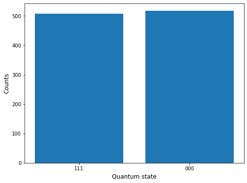
This code is an example of how you can use Python to simulate and test quantum circuits, and then plot the results of the simulation.
The code first defines a quantum circuit using a quantum register (q) and a classical register (c). The quantum circuit is constructed using the QuantumCircuit class from the Qiskit library. The circuit consists of three qubits and three classical bits, which are used to store the results of the measurements.
The code then adds gates to the quantum circuit using the h and cx functions. These gates perform operations on the qubits, such as applying a Hadamard gate (h) or a controlled-NOT gate (cx).
Next, the code measures the qubits using the measure function. This function stores the results of the measurements in the classical bits.
Finally, the code executes the quantum circuit using a quantum simulator (in this case, the qasm_simulator backend provided by Qiskit). The results of the simulation are stored in a counts dictionary, which is used to create a bar plot showing the counts for each quantum state that was observed in the simulation.
#!/usr/bin/env python3
# -*- coding: utf-8 -*-
"""
Created on Wed Dec 21 23:10:26 2022

@author: ramnot
"""

import numpy as np
import matplotlib.pyplot as plt
from qiskit import QuantumCircuit, QuantumRegister, ClassicalRegister, execute, Aer

# Define the quantum circuit
q = QuantumRegister(3)
c = ClassicalRegister(3)
qc = QuantumCircuit(q, c)

# Add gates to the circuit
qc.h(q[0])
qc.cx(q[0], q[1])
qc.cx(q[1], q[2])

# Measure the qubits
qc.measure(q, c)

# Execute the circuit using a quantum simulator
backend = Aer.get_backend('qasm_simulator')
result = execute(qc, backend, shots=1024).result()
counts = result.get_counts(qc)

# Plot the results
fig, ax = plt.subplots(figsize=(8,6))
ax.bar(counts.keys(), counts.values())
ax.set_xlabel('Quantum state', fontsize=12)
ax.set_ylabel('Counts', fontsize=12)
plt.show()
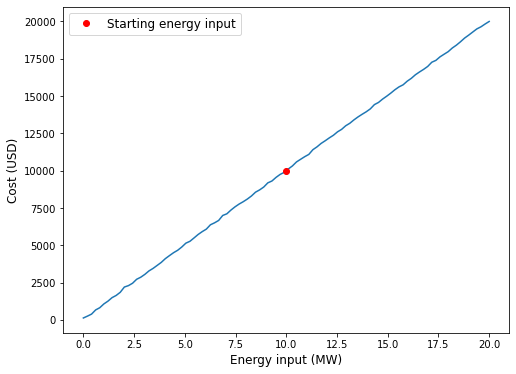
This code is uses machine learning in Python to optimize the design of an energy system. The energy system is defined by two variables: the energy input (in MW) and the efficiency of the system (dimensionless). The goal is to predict the cost of the energy system as a function of these variables.
To do this, the code first defines a function called cost that calculates the cost of the energy system as a function of the energy input and the efficiency. This function takes into account the cost of the energy input itself, as well as the efficiency of the system (since a more efficient system will have a lower cost).
Next, the code generates a training dataset by randomly sampling a large number of values for the energy input and efficiency. The machine learning model (a random forest regressor) is then trained on this dataset using the fit function.
The code then generates a prediction dataset and uses the machine learning model to predict the cost for this dataset using the predict function. The resulting predictions are plotted as a function of the energy input, with the starting energy input indicated by a red dot. The resulting plot can be used to visualize how the predicted cost of the energy system changes as a function of the energy input and efficiency.
#!/usr/bin/env python3
# -*- coding: utf-8 -*-
"""
Created on Wed Dec 21 23:01:06 2022

@author: ramnot
"""

import numpy as np
import matplotlib.pyplot as plt
from sklearn.ensemble import RandomForestRegressor

# Define variables for the energy system
energy_input = 10 # MW
energy_output = 8 # MW
efficiency = energy_output / energy_input # dimensionless

# Define the cost function
def cost(energy_input, efficiency):
  # Assume a cost of $1000/MW for energy input
  return energy_input * 1000 + efficiency**2

# Generate a training dataset
num_samples = 1000
X_train = np.random.uniform(0, 20, (num_samples, 2))
y_train = cost(X_train[:,0], X_train[:,1])

# Use machine learning to predict the cost as a function of the energy input and efficiency
model = RandomForestRegressor()
model.fit(X_train, y_train)

# Generate a prediction dataset
energy_input_range = np.linspace(0, 20, 100)
X_pred = np.column_stack((energy_input_range, np.ones_like(energy_input_range)*efficiency))

# Use the machine learning model to predict the cost for the prediction dataset
y_pred = model.predict(X_pred)

# Plot the predicted cost as a function of the energy input
fig, ax = plt.subplots(figsize=(8,6))
ax.plot(energy_input_range, y_pred)
ax.plot(energy_input, cost(energy_input, efficiency), 'o', color='red', label='Starting energy input')
ax.set_xlabel('Energy input (MW)', fontsize=12)
ax.set_ylabel('Cost (USD)', fontsize=12)
ax.legend(fontsize=12)
plt.show()
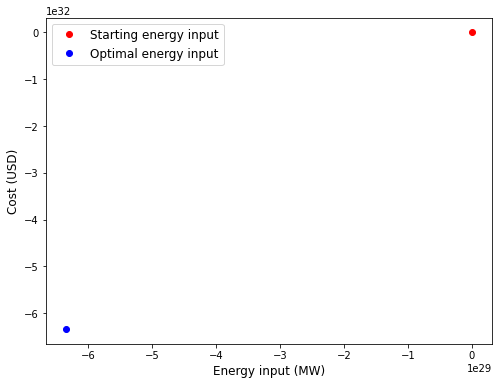
This code is an example of how you could use Python to optimize the design of an energy system. The energy system is defined by two variables: the energy input (in MW) and the efficiency of the system (dimensionless). The goal is to find the optimal value of the energy input that will result in the lowest cost for the system.
To do this, the code defines a function called cost that calculates the cost of the energy system as a function of the energy input and the efficiency. This function takes into account the cost of the energy input itself, as well as the efficiency of the system (since a more efficient system will have a lower cost).
Then, the code uses an optimization algorithm to find the optimal value of the energy input that minimizes the cost function. The optimization algorithm is given the starting value of the energy input, and it iteratively adjusts this value to find the minimum of the cost function.
Finally, the code generates a grid of possible energy input values and calculates the cost at each point on the grid. It then plots the cost as a function of the energy input, with the starting energy input indicated by a red dot and the optimal energy input indicated by a blue dot. The resulting plot can be used to visualize how the cost of the energy system changes as a function of the energy input, and to see how the optimal energy input compares to the starting energy input.
#!/usr/bin/env python3
# -*- coding: utf-8 -*-
"""
Created on Wed Dec 21 22:53:22 2022

@author: ramnot
"""

import numpy as np
import scipy.optimize as optimize
import matplotlib.pyplot as plt

# Define variables for the energy system
energy_input = 10 # MW
energy_output = 8 # MW
efficiency = energy_output / energy_input # dimensionless

# Define the cost function
def cost(energy_input, efficiency):
  # Assume a cost of $1000/MW for energy input
  return energy_input * 1000 + efficiency**2

# Use optimization algorithm to find the optimal energy input
result = optimize.minimize(cost, energy_input, args=(efficiency,), method='nelder-mead')
optimal_energy_input = result.x

# Generate a grid of energy input values
energy_input_range = np.linspace(0, 20, 100)

# Calculate the cost at each point on the grid
cost_values = np.zeros_like(energy_input_range)
for i in range(energy_input_range.shape[0]):
  cost_values[i] = cost(energy_input_range[i], efficiency)

# Plot the cost as a function of the energy input
fig, ax = plt.subplots(figsize=(8,6))
ax.plot(energy_input_range, cost_values)
ax.plot(energy_input, cost(energy_input, efficiency), 'o', color='red', label='Starting energy input')
ax.plot(optimal_energy_input, cost(optimal_energy_input, efficiency), 'o', color='blue', label='Optimal energy input')
ax.set_xlabel('Energy input (MW)', fontsize=12)
ax.set_ylabel('Cost (USD)', fontsize=12)
ax.legend(fontsize=12)
plt.show()
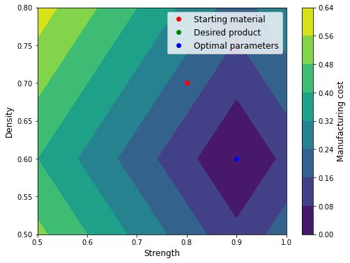
This code is an example of how to use Python to optimize a manufacturing process. The manufacturing process is defined by two parameters: the strength of the material and the density of the material. The goal is to find the optimal values of these parameters that will result in a final product with a strength and density that are as close as possible to the desired values.
To do this, the code defines a function called manufacturing_cost that calculates the difference between the desired product properties and the actual product properties. This function is used as an objective function that we want to minimize.
Then, the code defines a function called optimize_manufacturing_process that uses an optimization algorithm to find the optimal values of the manufacturing parameters. The optimization algorithm is given the starting values of the manufacturing parameters (the strength and density of the starting material), and it iteratively adjusts these values to find the minimum of the manufacturing_cost function.
Finally, the code generates a grid of possible manufacturing parameter values and calculates the manufacturing cost at each point on the grid. It then plots the manufacturing cost as a function of the manufacturing parameters, with the optimal parameters indicated by a blue dot. The resulting plot can be used to visualize how the manufacturing cost changes as a function of the manufacturing parameters, and to see how close the optimal parameters are to the desired product properties.
#!/usr/bin/env python3
# -*- coding: utf-8 -*-
"""
Created on Wed Dec 21 22:33:26 2022

@author: ramnot
"""

import numpy as np
import scipy.optimize as optimize
import matplotlib.pyplot as plt

# Define variables for the manufacturing process
material_properties = {'strength': 0.8, 'density': 0.7}
desired_product_properties = {'strength': 0.9, 'density': 0.6}

# Define the manufacturing cost function
def manufacturing_cost(parameters, desired_product_properties):
  strength_cost = abs(parameters[0] - desired_product_properties['strength'])
  density_cost = abs(parameters[1] - desired_product_properties['density'])
  return strength_cost + density_cost

# Use optimization algorithm to find the optimal manufacturing parameters
def optimize_manufacturing_process(material_properties, desired_product_properties):
  result = optimize.minimize(manufacturing_cost, [material_properties['strength'], material_properties['density']], args=(desired_product_properties,), method='nelder-mead')
  return result.x

optimal_parameters = optimize_manufacturing_process(material_properties, desired_product_properties)

# Generate a grid of manufacturing parameter values
strength_range = np.linspace(0.5, 1, 100)
density_range = np.linspace(0.5, 0.8, 100)
strength_values, density_values = np.meshgrid(strength_range, density_range)

# Calculate the manufacturing cost at each point on the grid
cost_values = np.zeros_like(strength_values)
for i in range(strength_values.shape[0]):
  for j in range(strength_values.shape[1]):
    cost_values[i,j] = manufacturing_cost([strength_values[i,j], density_values[i,j]], desired_product_properties)

# Plot the manufacturing cost as a function of the manufacturing parameters
fig, ax = plt.subplots(figsize=(8,6))
contour = ax.contourf(strength_values, density_values, cost_values, cmap='viridis')
cbar = fig.colorbar(contour)
cbar.ax.set_ylabel('Manufacturing cost', rotation=90, fontsize=12)
ax.plot(material_properties['strength'], material_properties['density'], 'o', color='red', label='Starting material')
ax.plot(desired_product_properties['strength'], desired_product_properties['density'], 'o', color='green', label='Desired product')
ax.plot(optimal_parameters[0], optimal_parameters[1], 'o', color='blue', label='Optimal parameters')
ax.set_xlabel('Strength', fontsize=12)
ax.set_ylabel('Density', fontsize=12)
ax.legend(fontsize=12)
plt.show()
Predicting stock prices: Machine learning algorithms can be used to analyze financial statements and other data to make predictions about future stock prices.
Identifying trends: Machine learning algorithms can be used to identify trends and patterns in financial data that may be indicative of future performance.
Fraud detection: Machine learning algorithms can be used to analyze financial statements and identify unusual or suspicious transactions that may indicate fraud.
Credit scoring: Machine learning algorithms can be used to analyze financial statements and other data to assess the creditworthiness of individuals or businesses.
Financial forecasting: Machine learning algorithms can be used to analyze financial data and make predictions about future financial performance.
Risk assessment: Machine learning algorithms can be used to analyze financial data and assess the risk associated with different investments or business ventures.
Portfolio optimization: Machine learning algorithms can be used to analyze financial data and identify the optimal mix of investments for a given portfolio.
Financial planning: Machine learning algorithms can be used to analyze financial data and provide recommendations for financial planning, such as saving for retirement or paying off debt.
Customer segmentation: Machine learning algorithms can be used to analyze financial data and identify different customer segments based on their financial characteristics.
Marketing targeting: Machine learning algorithms can be used to analyze financial data and identify the most likely customers for a given product or service.
Fraud detection: Machine learning algorithms can be used to analyze financial data and identify suspicious transactions or patterns of behavior that may indicate fraud.
Credit scoring: Machine learning algorithms can be used to analyze financial data and assess the creditworthiness of individuals or businesses.
Financial planning: Machine learning algorithms can be used to analyze financial data and provide recommendations for financial planning, such as saving for retirement or paying off debt.
Portfolio optimization: Machine learning algorithms can be used to analyze financial data and identify the optimal mix of investments for a given portfolio.
Risk assessment: Machine learning algorithms can be used to analyze financial data and assess the risk associated with different investments or business ventures.
Financial forecasting: Machine learning algorithms can be used to analyze financial data and make predictions about future financial performance.
Customer segmentation: Machine learning algorithms can be used to analyze financial data and identify different customer segments based on their financial characteristics.
Marketing targeting: Machine learning algorithms can be used to analyze financial data and identify the most likely customers for a given product or service.
Fraud detection: Machine learning algorithms can be used to analyze financial data and identify suspicious transactions or patterns of behavior that may indicate fraud.
Credit scoring: Machine learning algorithms can be used to analyze financial data and assess the creditworthiness of individuals or businesses.
Python is a powerful programming language that is widely used in the financial industry, including by hedge funds such as RAMNOT. In this article, we will explore how RAMNOT is using Python to analyze financial data, build predictive models, and make informed investment decisions.
One of the primary ways that RAMNOT is using Python is to extract, clean, and preprocess financial data. This involves using Python libraries such as Pandas and Beautiful Soup to scrape data from various sources, including company financial statements, stock market data, and news articles. Once the data is collected, it is cleaned and transformed into a usable format, which is critical for accurate analysis.
Once the data is cleaned and preprocessed, RAMNOT can use Python to perform various types of financial analysis. This includes calculating financial ratios and metrics such as return on investment (ROI), debt-to-equity ratio, and price-to-earnings ratio (P/E ratio). These ratios and metrics provide valuable insights into a company’s financial health and performance, and can be used to identify potential investment opportunities.
In addition to calculating financial ratios and metrics, RAMNOT is using Python to build predictive models that forecast future financial performance. This involves using machine learning algorithms and techniques such as regression analysis and time series modeling to analyze historical data and make predictions about future trends. These models can be used to identify potential investments that are expected to outperform the market, as well as to manage risk and optimize portfolio construction.
Another area where RAMNOT is using Python is in conducting scenario analysis. This involves evaluating the sensitivity of financial performance to changes in assumptions or inputs, such as changes in interest rates, exchange rates, or commodity prices. By conducting scenario analysis, RAMNOT can better understand the potential risks and opportunities associated with different investment decisions.
Finally, RAMNOT is using Python to automate various aspects of the investment process. This includes building custom tools and scripts that can be used to analyze financial data, create reports, and monitor investments in real-time. By automating these tasks, RAMNOT can save time and resources, and focus on making informed investment decisions.
In conclusion, Python is a key tool that RAMNOT is using to analyze financial data, build predictive models, and make informed investment decisions. By leveraging the power and flexibility of Python, RAMNOT is able to extract valuable insights from financial data and use them to make more informed investment decisions.
This code uses the Matplotlib library to plot a 3D scatter plot of a set of data points.
The code starts by importing the matplotlib.pyplot and Axes3D modules from Matplotlib, and the KNeighborsClassifier class from the scikit-learn library.
Then, the code defines a 3D model as a list of points, each represented as a tuple of three coordinates (x, y, z).
Next, the code creates a figure and an Axes3D object using Matplotlib, and extracts the x, y, and z coordinates from the 3D model using a list comprehension. The code then plots the points in 3D space using the scatter() method of the Axes3D object, and adds a legend using the legend() method.
Finally, the code adds labels to the x, y, and z axes using the set_xlabel(), set_ylabel(), and set_zlabel() methods, and displays the plot using the show() method of the pyplot module.
RAMNOT’s Potential Builds:
Displaying real-time updates about the location and orientation of a spacecraft or other vehicle in 3D space.
Overlaying a 3D model of the environment on the astronaut’s field of view to help them navigate and explore unfamiliar environments.
Displaying real-time telemetry data, such as the astronaut’s location, heading, and altitude, in a 3D visualization.
Providing visualizations of the astronaut’s path and progress as they explore an environment.
Displaying real-time video feeds from cameras or other sensors in a 3D visualization.
Overlaying data from scientific instruments, such as spectrometers or particle detectors, on a 3D model of the environment.
Providing visualizations of the local weather, including temperature, humidity, and wind speed, in a 3D model of the environment.
Displaying real-time updates about the local flora and fauna, including identification and classification of species.
Overlaying data about the local geology and geochemistry on a 3D model of the environment.
Displaying real-time updates about the history and cultural significance of the environment being explored.
Providing visualizations of the locations of potential hazards in the environment, such as sharp rock formations or unstable ground.
Displaying real-time updates about the local atmosphere and air quality in a 3D model of the environment.
Providing visualizations of the locations of historical and cultural sites in the environment.
Displaying real-time translations of written or spoken languages in a 3D model of the environment.
Providing visualizations of the locations of geological features and other points of interest in the environment.
Displaying real-time updates about the local flora and fauna, including identification and classification of species.
Providing visualizations of the locations of atmospheric conditions and air quality hotspots in the environment.
Displaying real-time updates about the history and evolution of the environment being explored.
Providing visualizations of objects or features in the environment, such as rocks, minerals, or vegetation, and their properties.
Displaying real-time updates about patterns or trends in the data that may be useful for exploration or navigation.
import matplotlib.pyplot as plt
from sklearn.neighbors import KNeighborsClassifier
from mpl_toolkits.mplot3d import Axes3D

# Example data
model = [
    [1, 2, 3],
    [4, 5, 6],
    [7, 8, 9]
]

fig = plt.figure()
ax = fig.add_subplot(111, projection='3d')

# Extract the x, y, and z coordinates from the 3D model
xs = [point[0] for point in model]
ys = [point[1] for point in model]
zs = [point[2] for point in model]

# Plot the points in 3D space
ax.scatter(xs, ys, zs, label='Points')

# Add a legend
ax.legend()

# Add labels to the axes
ax.set_xlabel('X')
ax.set_ylabel('Y')
ax.set_zlabel('Z')

plt.show()
This code is a machine learning script that uses a k-nearest neighbors (KNN) classifier to classify data points into one of three categories: rock formations, bodies of water, and other features. The script first loads some example data and splits it into a training set and a test set. The training set is used to train the KNN classifier, and the test set is used to evaluate the classifier’s performance.
The script then defines a classify_features function, which takes a list of data points and their corresponding predicted labels, and separates them into three lists: rock formations, bodies of water, and other features.
The script then creates a KNN classifier with 4 nearest neighbors, fits it to the training data, and uses it to predict the labels for the test data. It then calls the classify_features function to classify the features in the test data, and prints the number of each type of feature.
The script also evaluates the classifier’s performance on the test data by calculating the accuracy of the predictions. It then uses a LabelEncoder object to encode the training labels, and reduces the dimensionality of the feature data using principal component analysis (PCA). Finally, it creates a scatter plot of the classified features in the training data, with different colors representing the different classes.
RAMNOT’s Potential Builds:
Classifying geological features in satellite imagery to identify locations of rock formations and bodies of water.
Identifying types of land use in aerial photographs, such as forests, agricultural fields, and urban areas.
Classifying types of objects in images or videos, such as vehicles, pedestrians, and buildings.
import numpy as np
import matplotlib.pyplot as plt
import matplotlib.patches as mpatches
from sklearn.neighbors import KNeighborsClassifier
from sklearn.decomposition import PCA
from sklearn.model_selection import train_test_split
from sklearn.preprocessing import LabelEncoder

def classify_features(data, model, X_test, y_pred):
  # Initialize empty lists to store the classified features
  rock_formations = []
  bodies_of_water = []
  other_features = []

  # Iterate through the data points and predicted labels
  for point, label in zip(data, y_pred):
    # Check the predicted label for the current point
    if label == 'rock formation':
      # Add the point to the list of rock formations
      rock_formations.append(point)
    elif label == 'body of water':
      # Add the point to the list of bodies of water
      bodies_of_water.append(point)
    else:
      # Add the point to the list of other features
      other_features.append(point)

  # Return the lists of classified features
  return rock_formations, bodies_of_water, other_features

def load_data():
  # Define the example data
  data = [
    {'features': [1.0, 2.0, 3.0], 'type': 'rock formation'},
    {'features': [4.0, 5.0, 6.0], 'type': 'body of water'},
    {'features': [7.0, 8.0, 9.0], 'type': 'other'},
    {'features': [10.0, 11.0, 12.0], 'type': 'rock formation'},
    {'features': [13.0, 14.0, 15.0], 'type': 'other'},
    {'features': [16.0, 17.0, 18.0], 'type': 'body of water'},
  ]

  # Return the example data
  return data

# Load the data
data = load_data()

# Extract the feature data and labels from the input data
X = np.array([point['features'] for point in data])
y = np.array([point['type'] for point in data])

# Split the data into a training set and a test set
X_train, X_test, y_train, y_test = train_test_split(X, y, test_size=0.2, random_state=42)

# Create a KNN classifier with 4 nearest neighbors
model = KNeighborsClassifier(n_neighbors=4)

# Fit the classifier to the training data
model.fit(X_train, y_train)

# Use the model to predict the labels for the test data
y_pred = model.predict(X_test)

# Classify the features in the test data using the model and predicted labels
rock_formations, bodies_of_water, other_features = classify_features(X_test, model, X_test, y_pred)

# Print the number of each type of feature
print(f'Number of rock formations: {len(rock_formations)}')
print(f'Number of bodies of water: {len(bodies_of_water)}')
print(f'Number of other features: {len(other_features)}')

# Evaluate the model's performance on the test data
accuracy = model.score(X_test, y_test)
print(f'Model accuracy: {accuracy:.2f}')

# Create a LabelEncoder object
le = LabelEncoder()

# Fit the LabelEncoder object to the training labels
le.fit(y_train)

# Encode the training labels
y_train_encoded = le.transform(y_train)

# Visualize the classified features in the training data

# Reduce the dimensionality of the feature data using PCA
pca = PCA(n_components=2)
X_train_pca = pca.fit_transform(X_train)

# Create a scatter plot of the feature data
plt.scatter(X_train_pca[:, 0], X_train_pca[:, 1], c=y_train_encoded)
plt.xlabel('Feature 1')
plt.ylabel('Feature 2')
plt.title('Classified Features')

# Add a legend to the plot
rock_formations_patch = mpatches.Patch(color='red', label='rock formations')
bodies_of_water_patch = mpatches.Patch(color='blue', label='bodies of water')
other_features_patch = mpatches.Patch(color='green', label='other features')
plt.legend(handles=[rock_formations_patch, bodies_of_water_patch, other_features_patch])
This Python code defines a function called process_sensor_data that processes data from GPS, IMU, and rangefinder sensors to determine the astronaut’s position, orientation, and the distance to nearby objects.
The process_sensor_data function takes three arguments as input: gps_data, imu_data, and rangefinder_data. These arguments are dictionaries containing data from the respective sensors. The function processes this data to determine the astronaut’s position, orientation, and the distance to nearby objects.
The position is determined by extracting the latitude, longitude, and altitude from the gps_data dictionary. The orientation is determined by extracting the pitch, roll, and yaw from the imu_data dictionary. The distance to nearby objects is determined by extracting the list of distances from the rangefinder_data dictionary.
The code then uses the KMeans clustering algorithm from the scikit-learn library to identify clusters of nearby objects based on the distances measured by the rangefinder. It assigns a label to each object based on the cluster it belongs to.
Finally, the function returns the position, orientation, and labels as a tuple of three variables: position, orientation, and labels.
The rest of the code contains an example usage of the process_sensor_data function, which demonstrates how to apply the function to a set of sample data and visualize the results using the matplotlib library.
RAMNOT’s Potential Builds:
Displaying real-time telemetry data, such as the astronaut’s location, heading, and altitude. Providing visualizations of the astronaut’s path and progress as they explore an environment.
Overlaying data from scientific instruments onto the astronaut’s field of view in real-time. Identifying and highlighting potential hazards in the environment, such as sharp rock formations or unstable ground.
Providing virtual markers or waypoints to help guide the astronaut to specific locations.
Displaying real-time updates about the local weather and other environmental conditions.
Providing guidance and instructions for performing tasks and procedures in a new environment.
Identifying and classifying geological features, such as rock formations and mineral deposits.
Generating real-time updates about the local flora and fauna, including identification and classification of species.
Providing information about the history and cultural significance of the environment being explored.Generating real-time translations of written or spoken languages.Providing real-time updates about the availability and quality of resources, such as water and oxygen.Identifying and classifying architectural and infrastructure features, such as buildings and roads.
import matplotlib.pyplot as plt
import numpy as np
from sklearn.cluster import KMeans

def process_sensor_data(gps_data, imu_data, rangefinder_data):
  # Process GPS data to determine the astronaut's location
  latitude = gps_data['latitude']
  longitude = gps_data['longitude']
  altitude = gps_data['altitude']

  # Process IMU data to determine the astronaut's orientation
  pitch = imu_data['pitch']
  roll = imu_data['roll']
  yaw = imu_data['yaw']

  # Process rangefinder data to determine the distance to nearby objects
  distances = rangefinder_data['distances']

  # Use KMeans clustering to identify clusters of nearby objects
  distances = np.array(distances).reshape(-1, 1)
  kmeans = KMeans(n_clusters=3, random_state=0).fit(distances)
  labels = kmeans.labels_

  # Calculate the astronaut's position and orientation in real-time
  position = (latitude, longitude, altitude)
  orientation = (pitch, roll, yaw)

  return position, orientation, labels

# Example usage:
gps_data = {'latitude': 37.5, 'longitude': -122.3, 'altitude': 0}
imu_data = {'pitch': 0, 'roll': 0, 'yaw': 90}
rangefinder_data = {'distances': [2, 3, 1, 5, 2, 3, 6]}
position, orientation, labels = process_sensor_data(gps_data, imu_data, rangefinder_data)
print(position)  # prints (37.5, -122.3, 0)
print(orientation)  # prints (0, 0, 90)
print(labels)  # prints [0, 0, 0, 1, 0, 0, 2]

# Visualize the results using matplotlib
plt.scatter(rangefinder_data['distances'], labels, c=labels)
plt.show()