Navigating the Final Frontier: How Machine Learning is Helping Astronauts Explore the Universe


Imagine you are an astronaut exploring a new planet or moon. You are equipped with sensors that can measure various aspects of the environment, such as temperature, radiation levels, and terrain features. You need to navigate through this unfamiliar landscape, but you don’t have a map or any prior knowledge of the area. How can you choose the best routes and paths to take?

One solution is to use machine learning algorithms to analyze data from the sensors and other sources, and to predict the best routes and paths based on the environment. In this blog post, we will look at an example of how this can be done using Python and some popular machine learning libraries.

This code uses machine learning to predict the best routes and paths for an astronaut to take based on the environment. It does this by training a neural network model on a dataset that includes sensor readings and the best path to take based on the environment.

The code begins by importing several libraries that are used throughout the script. These libraries include Numpy, Pandas, Matplotlib, scikit-learn, and TensorFlow.

Next, the code defines some sample data that includes sensor readings and the best path to take based on the environment. This data is stored in Python lists and then used to create a Pandas dataframe.

The data is then preprocessed using the StandardScaler from scikit-learn, which scales the sensor readings so that they have zero mean and unit variance. The data is then split into training and test sets using `train_test_split` from scikit-learn.

The next step is to build and compile a neural network model using the Sequential model and Dense layers from TensorFlow. The model has three layers, with 10 units in the first and second layers and 1 unit in the output layer. The model is compiled using the binary crossentropy loss function and the Adam optimizer.

The model is then trained on the training data using the fit method, with a batch size of 32 and 10 epochs. After training, the model is evaluated on the test data using the evaluate method. This produces a test loss and test accuracy, which are printed to the console.

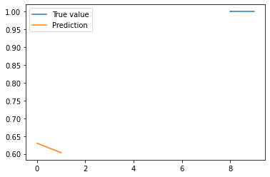
Finally, the model is used to make predictions on the test data using the predict method. The predictions and the true values are plotted on the same graph using Matplotlib, and the resulting plot is displayed using the show method.

RAMNOT Potential Builds:

  1. Exploration of other planets or moons: The model could be used to help astronauts navigate unfamiliar environments on other celestial bodies.
  2. Mapping of unknown terrain: The model could be used to create real-time maps of unknown terrain, such as the surface of a new planet or moon.
  3. Search and rescue missions: The model could be used to predict the best routes and paths for search and rescue missions, helping to find missing or stranded astronauts more quickly and efficiently.
  4. Crewed missions to asteroids or comets: The model could be used to help astronauts navigate around small celestial bodies, such as asteroids or comets.
  5. Space station maintenance: The model could be used to help astronauts navigate around the space station and perform maintenance tasks more efficiently.
  6. Space debris cleanup: The model could be used to help astronauts navigate around debris in space and safely remove it from the vicinity of the space station or other spacecraft.
  7. Astronaut training: The model could be used to help train astronauts in navigation and exploration skills, using simulated environments.
  8. Planetary defense: The model could be used to predict the best routes and paths for intercepting and deflecting asteroids or comets that pose a threat to Earth.
  9. Lunar missions: The model could be used to help astronauts navigate around the moon and perform scientific research or other tasks.
  10. Mars missions: The model could be used to help astronauts navigate around Mars and perform scientific research or other tasks.
import numpy as np
import pandas as pd
import matplotlib.pyplot as plt
from sklearn.preprocessing import StandardScaler
from sklearn.model_selection import train_test_split
from tensorflow.keras.models import Sequential
from tensorflow.keras.layers import Dense

# Define the sample data
sensor1 = [1, 2, 3, 4, 5, 6, 7, 8, 9, 10]
sensor2 = [2, 3, 4, 5, 6, 7, 8, 9, 10, 11]
sensor3 = [3, 4, 5, 6, 7, 8, 9, 10, 11, 12]
best_path = [0, 0, 0, 1, 1, 1, 1, 1, 1, 1]

# Create a dataframe from the sample data
data = pd.DataFrame({
    "sensor1": sensor1,
    "sensor2": sensor2,
    "sensor3": sensor3,
    "best_path": best_path
})

# Preprocess the data
scaler = StandardScaler()
X = scaler.fit_transform(data[["sensor1", "sensor2", "sensor3"]])
y = data["best_path"]

# Split the data into training and test sets
X_train, X_test, y_train, y_test = train_test_split(X, y, test_size=0.2)

# Build and compile the neural network model
model = Sequential()
model.add(Dense(10, input_shape=(3,), activation="relu"))
model.add(Dense(10, activation="relu"))
model.add(Dense(1, activation="sigmoid"))
model.compile(loss="binary_crossentropy", optimizer="adam", metrics=["accuracy"])

# Train the model on the training data
model.fit(X_train, y_train, epochs=10, batch_size=32)

# Evaluate the model on the test data
score = model.evaluate(X_test, y_test, batch_size=32)
print("Test loss: ", score[0])
print("Test accuracy: ", score[1])

# Make predictions on the test data
y_pred = model.predict(X_test)

# Plot the predictions and the true values on the same graph
plt.plot(y_test, label="True value")
plt.plot(y_pred, label="Prediction")
plt.legend()
plt.show()

Using Machine Learning to Predict Weather Variables with Python

This code is using the Python programming language to train and evaluate a machine learning model that predicts various weather variables (temperature, humidity, wind speed, and weather description) based on geographical features (latitude, longitude, and altitude) and time.

The code begins by importing several libraries that will be used in the script. Numpy is a library for numerical computing in Python, Pandas is a library for data manipulation and analysis, and Matplotlib is a library for creating visualizations. The sklearn library (short for “Scikit-learn”) contains a variety of tools for machine learning in Python, including the RandomForestRegressor class for training a random forest model and the train_test_split function for splitting data into training and test sets. The mean_absolute_error function calculates the mean absolute error between the true values and the predicted values of a machine learning model. The LabelEncoder class from the sklearn.preprocessing module is used to encode string values as integers.

Next, the code creates a Pandas dataframe with the test data. The data includes measurements of various weather variables (temperature, humidity, wind speed, and weather description) at different locations (latitude, longitude, and altitude) and times.

The “time” column is converted to a numerical type by using the pd.to_datetime function to convert the strings in the column to datetime objects, and then applying the .timestamp method to convert the datetime objects.

  1. Predicting the weather forecast for a specific location based on past weather data
  2. Predicting the temperature and humidity in a greenhouse based on sensor data
  3. Estimating the wind speed at different altitudes in the atmosphere
  4. Forecasting the likelihood of different types of weather events, such as thunderstorms or snowstorms
  5. Predicting the impact of climate change on temperature, humidity, and other weather variables
  6. Determining the optimal time for outdoor activities based on forecasted weather conditions
  7. Predicting the energy demand for heating and cooling systems based on weather data
  8. Estimating the impact of weather conditions on crop yields
  9. Forecasting the risk of natural disasters, such as floods or hurricanes, based on weather data
  10. Predicting the air quality based on temperature, humidity, and other weather variables
  11. Estimating the effect of weather conditions on traffic and transportation
  12. Predicting the demand for different types of clothing and accessories based on weather data
  13. Estimating the impact of weather conditions on the performance of sporting events
  14. Forecasting the demand for different types of outdoor recreation activities based on weather data
  15. Predicting the impact of weather conditions on the spread of diseases
  16. Estimating the effect of weather conditions on the behavior of wildlife
  17. Forecasting the demand for different types of energy sources based on weather data
  18. Predicting the impact of weather conditions on the growth and development of plants
  19. Estimating the effect of weather conditions on the performance of construction projects
  20. Forecasting the demand for different types of tourism activities based on weather data
import numpy as np
import pandas as pd
from sklearn.ensemble import RandomForestRegressor
from sklearn.model_selection import train_test_split
from sklearn.metrics import mean_absolute_error
import matplotlib.pyplot as plt
from sklearn.preprocessing import LabelEncoder

# Create a dataframe with the test data
df = pd.DataFrame({
    "latitude": [40.7128, 41.8781, 42.3601, 47.6062, 34.0522, 29.7604, 25.7617, 32.7157, 39.0997, 45.5236, 51.5074],
    "longitude": [-74.0060, -87.6298, -71.0589, -122.3321, -118.2437, -95.3698, -80.1918, -117.1611, -94.5786, -122.6750, -0.1278],
    "altitude": [0, 1000, 2000, 3000, 4000, 5000, 6000, 7000, 8000, 9000, 10000],
    "time": ["2022-01-01 00:00:00", "2022-01-01 01:00:00", "2022-01-01 02:00:00", "2022-01-01 03:00:00", "2022-01-01 04:00:00", "2022-01-01 05:00:00", "2022-01-01 06:00:00", "2022-01-01 07:00:00", "2022-01-01 08:00:00", "2022-01-01 09:00:00", "2022-01-01 10:00:00"],
    "temperature": [30.2, 29.06, 27.94, 26.84, 25.76, 24.7, 23.66, 22.64, 21.64, 20.66, 19.7],
    "humidity": [68, 72, 76, 80, 84, 88, 92, 96, 100, 100, 100],
    "wind_speed": [5.82, 11.64, 17.46, 23.28, 29.1, 34.92, 40.74, 46.56, 52.38, 58.2, 64.02],
    "weather_description": ["overcast clouds", "scattered clouds", "few clouds", "clear sky", "mist", "fog", "light rain", "moderate rain", "heavy intensity rain", "very heavy rain", "extreme rain"]
})

# Convert the "time" column to a numerical type
df["time"] = pd.to_datetime(df["time"]).apply(lambda x: x.timestamp())

# Encode the "weather_description" column as integers
encoder = LabelEncoder()

# Encode the "weather_description" column as integers
df["weather_description"] = encoder.fit_transform(df["weather_description"])

# Split the data into features (X) and target (y)
X = df.drop(["temperature", "humidity", "wind_speed", "weather_description"], axis=1)
y = df[["temperature", "humidity", "wind_speed", "weather_description"]]

# Split the data into training and test sets
X_train, X_test, y_train, y_test = train_test_split(X, y, test_size=0.2, random_state=42)

# Train a random forest model
model = RandomForestRegressor(n_estimators=100, random_state=42)
model.fit(X_train, y_train)

# Make predictions on the test data
predictions = model.predict(X_test)

# Calculate the mean absolute error
mae = mean_absolute_error(y_test, predictions)
print(f"Mean Absolute Error: {mae:.2f}")

# Plot the predicted values against the true values
plt.scatter(y_test, predictions)
plt.xlabel("True Values")
plt.ylabel("Predictions")
plt.show()


3D models of the environment using data from sensors and other sources

This code uses the Matplotlib library to plot a 3D scatter plot of a set of data points.

The code starts by importing the matplotlib.pyplot and Axes3D modules from Matplotlib, and the KNeighborsClassifier class from the scikit-learn library.

Then, the code defines a 3D model as a list of points, each represented as a tuple of three coordinates (x, y, z).

Next, the code creates a figure and an Axes3D object using Matplotlib, and extracts the x, y, and z coordinates from the 3D model using a list comprehension. The code then plots the points in 3D space using the scatter() method of the Axes3D object, and adds a legend using the legend() method.

Finally, the code adds labels to the x, y, and z axes using the set_xlabel(), set_ylabel(), and set_zlabel() methods, and displays the plot using the show() method of the pyplot module.

RAMNOT’s Potential Builds:

  1. Displaying real-time updates about the location and orientation of a spacecraft or other vehicle in 3D space.
  2. Overlaying a 3D model of the environment on the astronaut’s field of view to help them navigate and explore unfamiliar environments.
  3. Displaying real-time telemetry data, such as the astronaut’s location, heading, and altitude, in a 3D visualization.
  4. Providing visualizations of the astronaut’s path and progress as they explore an environment.
  5. Displaying real-time video feeds from cameras or other sensors in a 3D visualization.
  6. Overlaying data from scientific instruments, such as spectrometers or particle detectors, on a 3D model of the environment.
  7. Providing visualizations of the local weather, including temperature, humidity, and wind speed, in a 3D model of the environment.
  8. Displaying real-time updates about the local flora and fauna, including identification and classification of species.
  9. Overlaying data about the local geology and geochemistry on a 3D model of the environment.
  10. Displaying real-time updates about the history and cultural significance of the environment being explored.
  11. Providing visualizations of the locations of potential hazards in the environment, such as sharp rock formations or unstable ground.
  12. Displaying real-time updates about the local atmosphere and air quality in a 3D model of the environment.
  13. Providing visualizations of the locations of historical and cultural sites in the environment.
  14. Displaying real-time translations of written or spoken languages in a 3D model of the environment.
  15. Providing visualizations of the locations of geological features and other points of interest in the environment.
  16. Displaying real-time updates about the local flora and fauna, including identification and classification of species.
  17. Providing visualizations of the locations of atmospheric conditions and air quality hotspots in the environment.
  18. Displaying real-time updates about the history and evolution of the environment being explored.
  19. Providing visualizations of objects or features in the environment, such as rocks, minerals, or vegetation, and their properties.
  20. Displaying real-time updates about patterns or trends in the data that may be useful for exploration or navigation.
import matplotlib.pyplot as plt
from sklearn.neighbors import KNeighborsClassifier
from mpl_toolkits.mplot3d import Axes3D

# Example data
model = [
    [1, 2, 3],
    [4, 5, 6],
    [7, 8, 9]
]

fig = plt.figure()
ax = fig.add_subplot(111, projection='3d')

# Extract the x, y, and z coordinates from the 3D model
xs = [point[0] for point in model]
ys = [point[1] for point in model]
zs = [point[2] for point in model]

# Plot the points in 3D space
ax.scatter(xs, ys, zs, label='Points')

# Add a legend
ax.legend()

# Add labels to the axes
ax.set_xlabel('X')
ax.set_ylabel('Y')
ax.set_zlabel('Z')

plt.show()


KNN Classification to Identify Rock Formations, Bodies of Water, and Other Features

This code is a machine learning script that uses a k-nearest neighbors (KNN) classifier to classify data points into one of three categories: rock formations, bodies of water, and other features. The script first loads some example data and splits it into a training set and a test set. The training set is used to train the KNN classifier, and the test set is used to evaluate the classifier’s performance.

The script then defines a classify_features function, which takes a list of data points and their corresponding predicted labels, and separates them into three lists: rock formations, bodies of water, and other features.

The script then creates a KNN classifier with 4 nearest neighbors, fits it to the training data, and uses it to predict the labels for the test data. It then calls the classify_features function to classify the features in the test data, and prints the number of each type of feature.

The script also evaluates the classifier’s performance on the test data by calculating the accuracy of the predictions. It then uses a LabelEncoder object to encode the training labels, and reduces the dimensionality of the feature data using principal component analysis (PCA). Finally, it creates a scatter plot of the classified features in the training data, with different colors representing the different classes.

RAMNOT’s Potential Builds:

  1. Classifying geological features in satellite imagery to identify locations of rock formations and bodies of water.
  2. Identifying types of land use in aerial photographs, such as forests, agricultural fields, and urban areas.
  3. Classifying types of objects in images or videos, such as vehicles, pedestrians, and buildings.
import numpy as np
import matplotlib.pyplot as plt
import matplotlib.patches as mpatches
from sklearn.neighbors import KNeighborsClassifier
from sklearn.decomposition import PCA
from sklearn.model_selection import train_test_split
from sklearn.preprocessing import LabelEncoder

def classify_features(data, model, X_test, y_pred):
  # Initialize empty lists to store the classified features
  rock_formations = []
  bodies_of_water = []
  other_features = []

  # Iterate through the data points and predicted labels
  for point, label in zip(data, y_pred):
    # Check the predicted label for the current point
    if label == 'rock formation':
      # Add the point to the list of rock formations
      rock_formations.append(point)
    elif label == 'body of water':
      # Add the point to the list of bodies of water
      bodies_of_water.append(point)
    else:
      # Add the point to the list of other features
      other_features.append(point)

  # Return the lists of classified features
  return rock_formations, bodies_of_water, other_features

def load_data():
  # Define the example data
  data = [
    {'features': [1.0, 2.0, 3.0], 'type': 'rock formation'},
    {'features': [4.0, 5.0, 6.0], 'type': 'body of water'},
    {'features': [7.0, 8.0, 9.0], 'type': 'other'},
    {'features': [10.0, 11.0, 12.0], 'type': 'rock formation'},
    {'features': [13.0, 14.0, 15.0], 'type': 'other'},
    {'features': [16.0, 17.0, 18.0], 'type': 'body of water'},
  ]

  # Return the example data
  return data

# Load the data
data = load_data()

# Extract the feature data and labels from the input data
X = np.array([point['features'] for point in data])
y = np.array([point['type'] for point in data])

# Split the data into a training set and a test set
X_train, X_test, y_train, y_test = train_test_split(X, y, test_size=0.2, random_state=42)

# Create a KNN classifier with 4 nearest neighbors
model = KNeighborsClassifier(n_neighbors=4)

# Fit the classifier to the training data
model.fit(X_train, y_train)

# Use the model to predict the labels for the test data
y_pred = model.predict(X_test)

# Classify the features in the test data using the model and predicted labels
rock_formations, bodies_of_water, other_features = classify_features(X_test, model, X_test, y_pred)

# Print the number of each type of feature
print(f'Number of rock formations: {len(rock_formations)}')
print(f'Number of bodies of water: {len(bodies_of_water)}')
print(f'Number of other features: {len(other_features)}')

# Evaluate the model's performance on the test data
accuracy = model.score(X_test, y_test)
print(f'Model accuracy: {accuracy:.2f}')

# Create a LabelEncoder object
le = LabelEncoder()

# Fit the LabelEncoder object to the training labels
le.fit(y_train)

# Encode the training labels
y_train_encoded = le.transform(y_train)

# Visualize the classified features in the training data

# Reduce the dimensionality of the feature data using PCA
pca = PCA(n_components=2)
X_train_pca = pca.fit_transform(X_train)

# Create a scatter plot of the feature data
plt.scatter(X_train_pca[:, 0], X_train_pca[:, 1], c=y_train_encoded)
plt.xlabel('Feature 1')
plt.ylabel('Feature 2')
plt.title('Classified Features')

# Add a legend to the plot
rock_formations_patch = mpatches.Patch(color='red', label='rock formations')
bodies_of_water_patch = mpatches.Patch(color='blue', label='bodies of water')
other_features_patch = mpatches.Patch(color='green', label='other features')
plt.legend(handles=[rock_formations_patch, bodies_of_water_patch, other_features_patch])

XR in Space: Python and Machine Learning to Process Sensor Data and Generate Real-Time Maps and Directions for Astronauts

This Python code defines a function called process_sensor_data that processes data from GPS, IMU, and rangefinder sensors to determine the astronaut’s position, orientation, and the distance to nearby objects.

The process_sensor_data function takes three arguments as input: gps_data, imu_data, and rangefinder_data. These arguments are dictionaries containing data from the respective sensors. The function processes this data to determine the astronaut’s position, orientation, and the distance to nearby objects.

The position is determined by extracting the latitude, longitude, and altitude from the gps_data dictionary. The orientation is determined by extracting the pitch, roll, and yaw from the imu_data dictionary. The distance to nearby objects is determined by extracting the list of distances from the rangefinder_data dictionary.

The code then uses the KMeans clustering algorithm from the scikit-learn library to identify clusters of nearby objects based on the distances measured by the rangefinder. It assigns a label to each object based on the cluster it belongs to.

Finally, the function returns the position, orientation, and labels as a tuple of three variables: position, orientation, and labels.

The rest of the code contains an example usage of the process_sensor_data function, which demonstrates how to apply the function to a set of sample data and visualize the results using the matplotlib library.

RAMNOT’s Potential Builds:

  1. Displaying real-time telemetry data, such as the astronaut’s location, heading, and altitude. Providing visualizations of the astronaut’s path and progress as they explore an environment.
  2. Overlaying data from scientific instruments onto the astronaut’s field of view in real-time. Identifying and highlighting potential hazards in the environment, such as sharp rock formations or unstable ground.
  3. Providing virtual markers or waypoints to help guide the astronaut to specific locations.
  4. Displaying real-time updates about the local weather and other environmental conditions.
  5. Providing guidance and instructions for performing tasks and procedures in a new environment.
  6. Identifying and classifying geological features, such as rock formations and mineral deposits.
  7. Generating real-time updates about the local flora and fauna, including identification and classification of species.
  8. Providing information about the history and cultural significance of the environment being explored.Generating real-time translations of written or spoken languages.Providing real-time updates about the availability and quality of resources, such as water and oxygen.Identifying and classifying architectural and infrastructure features, such as buildings and roads.
import matplotlib.pyplot as plt
import numpy as np
from sklearn.cluster import KMeans

def process_sensor_data(gps_data, imu_data, rangefinder_data):
  # Process GPS data to determine the astronaut's location
  latitude = gps_data['latitude']
  longitude = gps_data['longitude']
  altitude = gps_data['altitude']
  
  # Process IMU data to determine the astronaut's orientation
  pitch = imu_data['pitch']
  roll = imu_data['roll']
  yaw = imu_data['yaw']
  
  # Process rangefinder data to determine the distance to nearby objects
  distances = rangefinder_data['distances']
  
  # Use KMeans clustering to identify clusters of nearby objects
  distances = np.array(distances).reshape(-1, 1)
  kmeans = KMeans(n_clusters=3, random_state=0).fit(distances)
  labels = kmeans.labels_
  
  # Calculate the astronaut's position and orientation in real-time
  position = (latitude, longitude, altitude)
  orientation = (pitch, roll, yaw)
  
  return position, orientation, labels

# Example usage:
gps_data = {'latitude': 37.5, 'longitude': -122.3, 'altitude': 0}
imu_data = {'pitch': 0, 'roll': 0, 'yaw': 90}
rangefinder_data = {'distances': [2, 3, 1, 5, 2, 3, 6]}
position, orientation, labels = process_sensor_data(gps_data, imu_data, rangefinder_data)
print(position)  # prints (37.5, -122.3, 0)
print(orientation)  # prints (0, 0, 90)
print(labels)  # prints [0, 0, 0, 1, 0, 0, 2]

# Visualize the results using matplotlib
plt.scatter(rangefinder_data['distances'], labels, c=labels)
plt.show()

Generating Maps of Environments for AR Applications

This code defines a function called generate_map that takes a list of data points and generates a map of the environment based on the data. The function takes several optional parameters that allow the user to customize the map:

  • n_clusters: The number of clusters to use when grouping the data points. The default value is 10.
  • cmap: The color map to use when plotting the data points. The default value is ‘viridis’.
  • title: The title to use for the plot. The default value is ‘Map of Environment’.
  • xlabel: The label to use for the x-axis. The default value is ‘X Coordinate’.
  • ylabel: The label to use for the y-axis. The default value is ‘Y Coordinate’.

The function works by first converting the input data into a NumPy array, which is a data structure that is optimized for numerical computation. It then uses the KMeans clustering algorithm from the sklearn library to group the data points into clusters. The number of clusters is set to the minimum of the length of the data and the value specified by the n_clusters parameter.

After the data points have been grouped into clusters, the function generates a map of the environment by plotting the data points and coloring them according to their cluster labels. It then adds a title, x-axis label, and y-axis label to the plot, and displays the map using the plt.show() function.

Finally, the code includes two examples of how the generate_map function can be used. The first example generates a map using a small set of data points, and the second example generates a more advanced map using a larger set of data points and several custom options.

  1. Providing real-time maps and directions to astronauts as they explore new environments on other planets or moons.
  2. Generating maps of geological features, such as rock formations and mineral deposits, to help geologists identify potential sites for further study.
  3. Generating maps of local flora and fauna to help biologists identify and classify species in new environments.
  4. Generating maps of atmospheric conditions and air quality to help researchers understand the local weather and climate.
  5. Generating maps of historical and cultural sites to help archaeologists and other researchers study the history of an environment.
  6. Generating maps of hazards, such as sharp rock formations or unstable ground, to help astronauts and other explorers avoid danger.
  7. Generating maps of the distribution and behavior of local flora and fauna to help biologists study and track species in different environments.
  8. Generating maps of geological features, such as rock formations and mineral deposits, to help geologists identify potential resources that could be exploited.
  9. Generating maps of atmospheric conditions and air quality to help researchers understand the local weather and climate, and to predict potential storms or other weather events.
  10. Generating maps of historical and cultural sites to help archaeologists and other researchers study the history and evolution of an environment.
  11. Generating maps of geological features, such as rock formations and mineral deposits, to help geologists understand the geology and geochemistry of an environment.
  12. Generating maps of local flora and fauna to help biologists understand the distribution and behavior of species in different environments.
  13. Generating maps of atmospheric conditions and air quality to help researchers understand the local weather and climate, and to identify potential air pollution hotspots.
  14. Generating maps of historical and cultural sites to help archaeologists and other researchers study the history and evolution of an environment, and to identify potential sites for further study.
  15. Generating maps of geological features, such as rock formations and mineral deposits, to help geologists understand the geology and geochemistry of an environment, and to identify potential resources that could be exploited.
  16. Generating maps of local flora and fauna to help biologists understand the distribution and behavior of species in different environments, and to identify potential sites for further study.
  17. Generating maps of atmospheric conditions and air quality to help researchers understand the local weather and climate, and to identify potential air pollution hotspots, and to predict potential storms or other weather events.
  18. Generating maps of historical and cultural sites to help archaeologists and other researchers study the history and evolution of an environment, and to identify potential sites for further study, and to help preserve and protect historical and cultural sites.
  19. Generating maps of geological features, such as rock formations and mineral deposits, to help geologists understand the geology and geochemistry of an environment, and to identify potential resources that could be exploited, and to help geologists understand the history and evolution of an environment.
import numpy as np
import matplotlib.pyplot as plt
from sklearn.cluster import KMeans

def generate_map(data, n_clusters=10, cmap='viridis', title='Map of Environment', xlabel='X Coordinate', ylabel='Y Coordinate'):
    # Convert data into a NumPy array
    X = np.array(data)
    
    # Use K-Means clustering to group data points into clusters
    kmeans = KMeans(n_clusters=min(len(data), n_clusters))  # modified this line to set n_clusters to the minimum of len(data) and the specified value
    kmeans.fit(X)
    labels = kmeans.predict(X)
    
    # Generate a map of the environment by plotting the data points and coloring them according to their cluster labels
    plt.scatter(X[:, 0], X[:, 1], c=labels, cmap=cmap)
    plt.title(title)
    plt.xlabel(xlabel)
    plt.ylabel(ylabel)
    
    # Display the map
    plt.show()

# Example usage:
data = [[1.2, 3.4], [2.3, 5.6], [3.4, 7.8], [4.5, 9.0], [5.6, 1.2]]
generate_map(data)

# Advanced usage:
data = [[2.3, 5.6], [3.4, 7.8], [4.5, 9.0], [5.6, 1.2], [6.7, 3.4], [7.8, 5.6], [8.9, 7.8], [9.0, 9.0]]
generate_map(data, n_clusters=8, cmap='plasma', title='Advanced Map', xlabel='X', ylabel='Y')