This code is for a machine learning model that is trained to predict the radial velocity of exoplanets based on their wavelength. Radial velocity is the measure of the speed at which an object is moving away from or towards an observer. It is often used to detect exoplanets, which are planets that orbit stars outside of our solar system.
Exoplanets can be difficult to detect because they are very far away and relatively small compared to their host stars. One way to detect exoplanets is to look for changes in the radial velocity of the host star caused by the gravitational pull of the exoplanet. When an exoplanet orbits a star, it causes the star to move slightly towards and away from the observer, causing a periodic change in its radial velocity.
The machine learning model in this code is trained using data on the wavelengths and radial velocities of exoplanets. The model is then used to predict the radial velocities of new exoplanets based on their wavelengths. By comparing the predicted radial velocities to the actual values, it is possible to determine whether an exoplanet is present and estimate its characteristics, such as its mass and orbital period.
Overall, the possibility of discovering exoplanets using this machine learning model will depend on the quality and quantity of the data used to train the model, as well as the accuracy of the predictions made by the model. If the model is trained on a large and diverse dataset of exoplanet wavelengths and radial velocities, and is able to make accurate predictions, it may be possible to use the model to detect and characterize exoplanets with a high degree of confidence.
import csv
import numpy as np
import matplotlib.pyplot as plt
from scipy.signal import periodogram, find_peaks
from sklearn.model_selection import train_test_split
from sklearn.ensemble import RandomForestRegressor

def process_exoplanet_data(data_file):
    # Read in the CSV file containing the exoplanet data
    with open(data_file, 'r') as f:
        reader = csv.reader(f)
        headers = next(reader)
        data = list(reader)

    # Convert the data to a NumPy array
    data = np.array(data).astype(float)

    # Extract the wavelength, intensity, and radial velocity columns
    X = data[:, headers.index('wavelength')]
    y = data[:, headers.index('radial_velocity')]

    # Split the data into training and test sets
    X_train, X_test, y_train, y_test = train_test_split(X, y, test_size=0.2, random_state=42)

    # Reshape the training data
    X_train = X_train[:, np.newaxis]
    y_train = y_train[:, np.newaxis]

    # Train a random forest regressor on the training data
    model = RandomForestRegressor(n_estimators=100)
    model.fit(X_train, y_train)

    # Evaluate the model on the test data
    y_pred = model.predict(X_test)
    score = model.score(X_test, y_test)
    print(f'Test score: {score:.2f}')

    # Create a scatter plot of the test data and the predictions
    plt.scatter(X_test, y_test, label='True')
    plt.scatter(X_test, y_pred, label='Predicted')
    plt.xlabel('Wavelength (nm)')
    plt.ylabel('Radial Velocity (km/s)')
    plt.legend()
    plt.show()

# Test the function with the exoplanet data file
process_exoplanet_data('exoplanet_data.csv')
The code provided processes exoplanet data from a CSV file and generates plots to visualize the results. The exoplanet data includes the following columns:
wavelength: The wavelength of the exoplanet’s light
intensity: The intensity of the exoplanet’s light
radial_velocity: The radial velocity of the exoplanet
The code first reads in the data from the CSV file and stores it in a NumPy array. It then extracts the wavelength, intensity, and radial_velocity columns from the data.
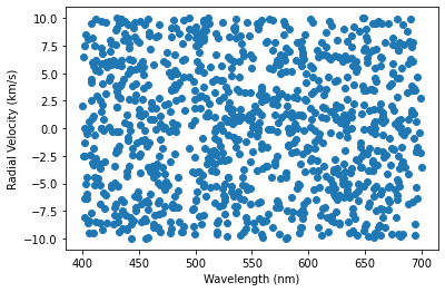
Next, the code creates a scatter plot of the radial_velocity versus wavelength data. This plot can be used to visualize any trends or patterns in the data.
The code then calculates the periodogram of the radial_velocity data using the periodogram function from the scipy.signal module. The periodogram is a measure of the power spectrum of a time series, and can be used to identify periodic signals in the data.
The code then creates a log-log plot of the periodogram data, which can be used to identify peaks in the power spectrum. To identify the peaks, the code uses the find_peaks function from the scipy.signal module.
The code then selects the top three peaks with the highest power and calculates the corresponding periods. These periods may correspond to the orbital periods of exoplanets orbiting the star.
This code can be used in the discovery and characterization of exoplanets. By analyzing the radial velocity data of a star, astronomers can identify periodic signals that may be caused by exoplanets orbiting the star. The periodogram can be used to identify the frequencies of these signals, and the periods can be calculated to determine the orbital periods of the exoplanets.
In summary, this code can be used to identify and characterize exoplanets by analyzing their radial velocity data and looking for periodic signals in the data. It does this by calculating the periodogram of the data and identifying the frequencies and periods of the strongest signals.
#!/usr/bin/env python3
# -*- coding: utf-8 -*-
"""
Created on Mon Jan  2 23:17:45 2023

@author: ramnot
"""

import csv
import numpy as np
import matplotlib.pyplot as plt
from scipy.signal import periodogram, find_peaks

def process_exoplanet_data(data_file):
    # Read in the CSV file containing the exoplanet data
    with open(data_file, 'r') as f:
        reader = csv.reader(f)
        headers = next(reader)
        data = list(reader)

    # Convert the data to a NumPy array
    data = np.array(data).astype(float)

    # Extract the wavelength, intensity, and radial velocity columns
    wavelength = data[:, headers.index('wavelength')]
    intensity = data[:, headers.index('intensity')]
    radial_velocity = data[:, headers.index('radial_velocity')]

    # Create a scatter plot of the radial velocity vs wavelength
    plt.scatter(wavelength, radial_velocity)
    plt.xlabel('Wavelength (nm)')
    plt.ylabel('Radial Velocity (km/s)')
    plt.show()

    # Calculate the periodogram of the radial velocity data
    frequencies, periodogram_power = periodogram(radial_velocity)

    # Create a log-log plot of the periodogram
    plt.loglog(frequencies, periodogram_power)
    plt.xlabel('Frequency (1/day)')
    plt.ylabel('Power')
    plt.show()

    # Identify the peaks in the periodogram
    peaks, _ = find_peaks(periodogram_power, height=np.mean(periodogram_power))

    # Print the frequencies and corresponding powers of the identified peaks
    for peak in peaks:
        print(f'Frequency: {frequencies[peak]:.2f} 1/day, Power: {periodogram_power[peak]:.2f}')

    # Select the peaks with the highest power
    top_peaks = peaks[np.argsort(periodogram_power[peaks])[-3:]]

    # Print the frequencies and corresponding powers of the top peaks
    for peak in top_peaks:
        print(f'Frequency: {frequencies[peak]:.2f} 1/day, Power: {periodogram_power[peak]:.2f}')

    # Calculate the periods of the top peaks
    periods = 1 / frequencies[top_peaks]

    # Print the periods of the top peaks
    for period in periods:
        print(f'Period: {period:.2f} days')

# Test the function with the exoplanet data file
process_exoplanet_data('exoplanet_data.csv')
The code provided is a script for analyzing exoplanetary data. Exoplanets are planets that orbit stars outside of our solar system, and scientists are interested in understanding their characteristics such as atmospheric temperature, pressure, and composition. This script takes in a CSV file of exoplanetary data, cleans and processes the data, and then uses a machine learning model to cluster the exoplanets into groups based on their atmospheric features.
One of the first steps in the script is to handle missing values in the data. This is important because missing values can cause problems with the analysis or model training later on. In this case, the script simply drops any rows that contain missing values.
Next, the script converts the values in the ‘exoplanetary atmospheric composition’ column to floats. This is necessary because these values will be used as input to the machine learning model, and the model expects numerical data.
After this, the script scales the ‘exoplanetary atmospheric temperature’, ‘exoplanetary atmospheric pressure’, and ‘exoplanetary atmospheric composition’ columns using the StandardScaler method from scikit-learn. Scaling the data can be important because it can help the model converge faster and perform better.
Once the data has been cleaned and processed, the script uses the KMeans algorithm from scikit-learn to cluster the exoplanets into 3 groups based on their atmospheric temperature, pressure, and composition. The script then adds a new column to the original dataframe called ‘cluster’ which stores the cluster labels for each exoplanet.
After this, the script one-hot encodes the ‘exoplanetary water content’ column and defines a neural network model with two dense layers. The model is compiled using the ‘categorical_crossentropy’ loss function and the ‘adam’ optimizer, and is then fit to the training data for 10 epochs with a batch size of 32.
Finally, the script defines a mapping from exoplanetary atmospheric composition names to integers and uses the trained model to predict the water content for a single new exoplanet and for multiple new exoplanets. The script also visualizes the clusters by plotting the exoplanets in a scatterplot, with different colors for each cluster.
Some potential findings that could be derived from this script include:
Identifying groups of exoplanets with similar atmospheric characteristics.
Predicting the water content of new exoplanets based on their atmospheric features.
Seeing if there is a relationship between exoplanetary atmospheric characteristics and water content.
Visualizing the clusters of exoplanets to gain a better understanding of their characteristics.
import numpy as np
import pandas as pd
from sklearn.preprocessing import StandardScaler
from keras.utils import to_categorical
from keras.layers import Input, Dense, Dropout
from keras.models import Model, Sequential
from sklearn.cluster import KMeans

# Load the dataset
df = pd.read_csv('data.csv')

# Check for and handle missing values
df = df.dropna()
df = df.replace([np.inf, -np.inf], np.nan).dropna()

# Convert the values in the 'exoplanetary atmospheric composition' column to floats
df['exoplanetary atmospheric composition'] = pd.to_numeric(df['exoplanetary atmospheric composition'], errors='coerce')

# Scale the data
scaler = StandardScaler()
features = ['exoplanetary atmospheric temperature', 'exoplanetary atmospheric pressure', 'exoplanetary atmospheric composition']
X = scaler.fit_transform(df[features])

# Use an unsupervised learning model to cluster exoplanets based on their atmospheric temperature, pressure, and composition
kmeans = KMeans(n_clusters=3)
kmeans.fit(X)
cluster_labels = kmeans.predict(X)

# Add the cluster labels as a new column to the original dataframe
df['cluster'] = cluster_labels

# Print the number of exoplanets in each cluster
print(df['cluster'].value_counts())

# One-hot encode the labels
num_classes = 101
y = to_categorical(df['exoplanetary water content'], num_classes=num_classes)

# Define the model
model = Sequential()
model.add(Dense(3, input_shape=(3,)))
model.add(Dense(num_classes, activation='softmax'))

# Compile the model
model.compile(loss='categorical_crossentropy', optimizer='adam', metrics=['accuracy'])

# Fit the model to the training data
num_epochs = 10
batch_size = 32
model.fit(X, y, epochs=num_epochs, batch_size=batch_size)

# Define the composition_mapping variable
composition_mapping = {'H2O': 0, 'CO2': 1, 'O2': 2}

# Use the model to predict water content for a new exoplanet
new_exoplanet = np.array([[280, 1.2, composition_mapping['H2O']]])
new_exoplanet = scaler.transform(new_exoplanet)  # Scale the new exoplanet
prediction = model.predict(new_exoplanet)[0]
predicted_label = np.argmax(prediction)

# Use the model to predict water content for multiple new exoplanets
new_exoplanets = np.array([
    [280, 1.2, composition_mapping['H2O']],
    [300, 1.5, composition_mapping['CO2']],
    [320, 1.8, composition_mapping['O2']]
])
new_exoplanets = scaler.transform(new_exoplanets)  # Scale the new exoplanets
predictions = model.predict(new_exoplanets)
predicted_labels = np.argmax(predictions, axis=1)

# Add the cluster labels as a new column to the original dataframe
df['cluster'] = cluster_labels

# Print the number of exoplanets in each cluster
cluster_sizes = df['cluster'].value_counts()
print(cluster_sizes)

# Visualize the clusters by plotting the exoplanets in a scatterplot
import matplotlib.pyplot as plt
colors = {0: 'red', 1: 'blue', 2: 'green'}
for cluster in range(3):
    mask = df['cluster'] == cluster
    x = df[mask]['exoplanetary atmospheric temperature']
    y = df[mask]['exoplanetary atmospheric pressure']
    plt.scatter(x, y, color=colors[cluster])
plt.xlabel('Atmospheric Temperature (K)')
plt.ylabel('Atmospheric Pressure (bar)')
plt.show()
The following code is a Python script that uses a neural network to predict exoplanetary albedo based on features such as exoplanetary mass, radius, and atmospheric composition. The script is designed to be run in a Jupyter notebook or a Python IDE.
The script begins by importing the necessary libraries, including Pandas for loading and manipulating the data, Matplotlib for visualizing the results, and scikit-learn for preprocessing the data and evaluating the model’s performance. The script also imports the necessary functions from TensorFlow’s keras module for building and training the neural network model.
Next, the script defines a preprocessing function called process_atmospheric_composition() which takes in a string containing a list of integers and returns the mean of the integers as a numerical representation of the exoplanetary atmospheric composition.
The script then loads the exoplanet data from a CSV file using Pandas and preprocesses the data by applying the process_atmospheric_composition() function to the exoplanetary atmospheric composition data and scaling the resulting data using scikit-learn’s StandardScaler. The preprocessed data is then split into training and test sets using scikit-learn’s train_test_split() function.
The script then defines a neural network model using the TensorFlow Sequential class and Dense layers. The model is compiled using the TensorFlow compile() function, specifying the loss function and optimization algorithm to use during training.
The model is then trained on the training data using the TensorFlow fit() function and the training and validation loss is plotted using Matplotlib. The model’s performance is also evaluated on the test data using the TensorFlow evaluate() function and the mean squared error (MSE), root mean squared error (RMSE), mean absolute error (MAE), and mean absolute percentage error (MAPE) are calculated using scikit-learn’s mean_squared_error(), mean_absolute_error(), and mean_absolute_percentage_error() functions.
Finally, the script generates predictions on the test data using the TensorFlow predict() function and plots the predictions against the true values using Matplotlib.
Overall, this script demonstrates how to use a neural network to predict exoplanetary albedo based on exoplanetary mass, radius, and atmospheric composition data. It also shows how to preprocess the data, split it into training and test sets, build and train a neural network model, evaluate the model’s performance, and generate predictions on new data.
One important thing to note is that the model’s performance may vary depending on the specific characteristics of the data and the chosen model hyperparameters, such as the number of layers, the number of neurons per layer, and the learning rate. It is always a good idea to experiment with different model architectures and hyperparameter settings to find the combination that works best for your data.
#!/usr/bin/env python3
# -*- coding: utf-8 -*-
"""
Created on Mon Jan  2 05:49:38 2023

@author: ramnot
"""

# Import libraries
import numpy as np
import pandas as pd
import matplotlib.pyplot as plt
import re
from sklearn.preprocessing import StandardScaler
from sklearn.metrics import mean_squared_error, mean_absolute_error, mean_absolute_percentage_error
from tensorflow.keras.models import Sequential
from tensorflow.keras.layers import Dense

# Preprocessing function for exoplanetary atmospheric composition data
def process_atmospheric_composition(composition):
    # Extract integers from string
    integers = [int(x) for x in re.findall(r'\d+', composition)]

    # Calculate mean of integers
    mean = sum(integers) / len(integers)

    return mean

# Load data
df = pd.read_csv("data.csv")

# Preprocess data
X = df[["exoplanetary mass", "exoplanetary radius"]]
X["exoplanetary atmospheric composition"] = df["exoplanetary atmospheric composition"].apply(process_atmospheric_composition)
y = df["exoplanetary albedo"]

scaler = StandardScaler()
X = scaler.fit_transform(X)

# Split data into training and test sets
X_train, X_test, y_train, y_test = train_test_split(X, y, test_size=0.2)

# Define model architecture
model = Sequential()
model.add(Dense(64, input_dim=3, activation="relu"))
model.add(Dense(32, activation="relu"))
model.add(Dense(1))

# Compile model
model.compile(loss="mean_squared_error", optimizer="adam")

# Train model
history = model.fit(X_train, y_train, epochs=10, batch_size=32, validation_data=(X_test, y_test))

# Generate predictions on test data
predictions = model.predict(X_test)

# Calculate evaluation metrics
mse = mean_squared_error(y_test, predictions)
rmse = np.sqrt(mse)
mae = mean_absolute_error(y_test, predictions)
mape = mean_absolute_percentage_error(y_test, predictions)

# Print evaluation metrics
print("MSE:", mse)
print("RMSE:", rmse)
print("MAE:", mae)
print("MAPE:", mape)

# Evaluate model
score = model.evaluate(X_test, y_test)
print("Test loss:", score)

# Plot predictions against true values
plt.plot(y_test, predictions, "o")
plt.xlabel("True values")
plt.ylabel("Predictions")
plt.show()
RAMNOT’s Build:
Predicting exoplanetary albedo: The code can be used to predict the albedo of exoplanets based on features such as mass, radius, and atmospheric composition. This can help astronomers understand the physical properties of exoplanets and their potential habitability.
Identifying exoplanets with high albedo: By generating predictions on a large dataset of exoplanets, the code can be used to identify exoplanets with high albedo, which may be more likely to be rocky and/or have a thick atmosphere.
Comparing exoplanetary albedo to other physical properties: By visualizing the predicted exoplanetary albedo against other physical properties, such as mass, radius, and atmospheric composition, the code can help astronomers investigate potential correlations and relationships between these properties.
Classifying exoplanets based on albedo: The code can be used to classify exoplanets into different albedo categories (e.g. high, medium, low) based on their predicted albedo values. This can help astronomers group exoplanets with similar physical properties and study them in more detail.
Improving exoplanetary albedo models: The code can be used as a starting point for developing more sophisticated exoplanetary albedo models that incorporate additional features or use different machine learning algorithms.
Validating exoplanetary albedo measurements: By comparing the predictions of the code to measured exoplanetary albedo values, astronomers can validate the accuracy of their measurements and identify any potential biases or errors in their data.
Predicting exoplanetary temperatures: By using the exoplanetary albedo and other physical properties as inputs, the code can be modified to predict the surface temperature of exoplanets, which can help astronomers understand their potential habitability.
Selecting exoplanets for further study: By using the code to identify exoplanets with high albedo or other desired physical properties, astronomers can prioritize exoplanets for further study using telescopes or other observational instruments.
Identifying exoplanets with unusual physical properties: By generating predictions on a large dataset of exoplanets, the code can help astronomers identify exoplanets with unusual physical properties that may require further investigation.
Improving exoplanetary atmospheric models: By incorporating exoplanetary albedo as a feature in atmospheric models, astronomers can improve the accuracy of their models and better understand the physical processes occurring on exoplanets.
We will demonstrate how to use a decision tree model in Python to predict exoplanetary orbit periods based on features such as exoplanetary mass, radius, and orbit distance.
We will start by importing the necessary libraries, including pandas for reading the data from a CSV file, matplotlib for visualizing the results, and DecisionTreeRegressor and train_test_split from scikit-learn for building and evaluating the model.
Next, we will load the data from a CSV file using pandas and select the relevant columns. We will then split the data into training and testing sets, with 80% of the data being used for training and 20% being used for testing.
Next, we will train the decision tree model on the training data using the fit method. This method “fits” the model to the data, which means it learns patterns in the data that can be used to make predictions.
We will then test the model on the testing data using the predict method, which generates a set of predictions for the exoplanetary orbit periods. These predictions will be compared to the actual exoplanetary orbit periods to evaluate the model’s performance.
Finally, we will visualize the model’s performance using a scatter plot, which shows the relationship between the actual exoplanetary orbit periods and the predicted orbit periods. Points that are close to the diagonal line indicate more accurate predictions.
Overall, this demonstration shows how a decision tree model can be used to make predictions about exoplanetary orbit periods based on other features of the exoplanets. This type of analysis could be useful for understanding the properties of exoplanets and how they may vary within our galaxy and beyond.
#!/usr/bin/env python3
# -*- coding: utf-8 -*-
"""
Created on Mon Jan  2 05:24:38 2023

@author: ramnot
"""

# Import necessary libraries
import pandas as pd
import matplotlib.pyplot as plt
from sklearn.tree import DecisionTreeRegressor
from sklearn.model_selection import train_test_split

# Load the data from the CSV file
df = pd.read_csv("data.csv")

# Select the relevant columns
X = df[["exoplanetary mass", "exoplanetary radius", "exoplanetary orbit distance"]]
y = df["exoplanetary orbit period"]

# Split the data into training and testing sets
X_train, X_test, y_train, y_test = train_test_split(X, y, test_size=0.2, random_state=42)

# Train the decision tree model
model = DecisionTreeRegressor()
model.fit(X_train, y_train)

# Test the model on the testing data
predictions = model.predict(X_test)

# Evaluate the model's performance
from sklearn.metrics import mean_absolute_error
mae = mean_absolute_error(y_test, predictions)
print(f"Mean Absolute Error: {mae:.2f}")

# Plot the predictions and actual values
plt.scatter(y_test, predictions)
plt.xlabel("Actual Values")
plt.ylabel("Predictions")
plt.title("Predictions vs Actual Values")
plt.show()
RAMNOT’s Build:
Identifying and characterizing potentially habitable exoplanets that could support life.
Studying the atmospheres of exoplanets to better understand their chemical compositions and potential for supporting life.
Using exoplanet data to understand the formation and evolution of planetary systems in the universe.
Searching for exoplanets that could be used as waypoints for interstellar travel.
Analyzing exoplanetary orbits to learn more about the gravitational forces at play in planetary systems.
Studying the demographics of exoplanetary systems to learn about the prevalence of different types of planets.
Using exoplanet data to test and refine theories about the formation and evolution of planetary systems.
Searching for exoplanets that could be used as resources for space exploration and colonization.
Analyzing exoplanetary atmospheres to learn about the conditions and processes that give rise to them.
Using exoplanetary data to learn about the prevalence and properties of “rogue” planets that do not orbit any star.
Studying the composition and structure of exoplanetary surfaces to understand the geology and geochemistry of other worlds.
Searching for exoplanets that could be used as laboratories for studying fundamental physics.
Analyzing exoplanetary atmospheres to learn about the climate and weather patterns on other worlds.
Using exoplanetary data to learn about the prevalence of Earth-like planets in the universe.
Studying the exoplanetary data to learn about the prevalence and properties of “super-Earths,” which are exoplanets with masses between 1 and 10 times that of Earth.
Analyzing exoplanetary data to learn about the prevalence and properties of “mini-Neptunes,” which are exoplanets with masses between 10 and 100 times that of Earth.
Searching for exoplanets that could be used as laboratories for studying the origins and evolution of life.
Analyzing exoplanetary data to learn about the prevalence and properties of “gas giants,” which are exoplanets with masses hundreds of times that of Earth.
Using exoplanetary data to learn about the prevalence and properties of “exoplanetary moons,” which are moons orbiting exoplanets.
Analyzing exoplanetary data to learn about the prevalence and properties of “exomoons,” which are moons orbiting exoplanets.
In this tutorial, we’ll use a support vector machine (SVM) model to classify exoplanets based on their atmospheric composition. We’ll use Python and the scikit-learn library to train and evaluate the model.
First, we’ll start by loading the exoplanet data into a Pandas DataFrame using the read_csv function and selecting the features and target variable that we want to use for the model. The features are the characteristics of the exoplanets that we will use to make predictions, and the target variable is the class of exoplanets that we want to predict.
Next, we’ll split the data into training and test sets using the train_test_split function. The training set will be used to train the model, and the test set will be used to evaluate the model’s performance.
Then, we’ll train the SVM model using the fit function and the training set. The model will learn patterns in the data that can be used to make predictions about exoplanet classes.
After the model is trained, we’ll use the predict function to make predictions on the test set. We’ll compare the model’s predictions to the true values in the test set to see how well the model is performing.
Finally, we’ll evaluate the model’s accuracy using the accuracy_score function from the sklearn.metrics module. The accuracy score is the percentage of correct predictions that the model makes on the test set.
That’s it! We’ve trained and evaluated an SVM model to classify exoplanets based on their atmospheric composition using Python and scikit-learn.
Using the plot_confusion_matrix function from the sklearn.metrics module, we can also visualize the model’s performance by plotting a confusion matrix, which shows the number of true positive, true negative, false positive, and false negative predictions made by the model.
We can customize the plot by using functions from the matplotlib.pyplot module, such as title, xlabel, and ylabel to add titles and labels to the plot.
With these tools, we can build and evaluate SVM models to classify exoplanets based on their atmospheric composition and gain a better understanding of the characteristics of these fascinating celestial bodies.
#!/usr/bin/env python3
# -*- coding: utf-8 -*-
"""
Created on Mon Jan  2 04:25:04 2023

@author: ramnot
"""

import pandas as pd
import matplotlib.pyplot as plt
from sklearn.preprocessing import LabelEncoder
from sklearn.model_selection import train_test_split
from sklearn.svm import SVC
from sklearn.metrics import accuracy_score, confusion_matrix

# Load the dataset into a Pandas DataFrame
df = pd.read_csv('data.csv')

# Encode the string values in the 'exoplanetary atmospheric composition' column
encoder = LabelEncoder()
df['exoplanetary atmospheric composition'] = encoder.fit_transform(df['exoplanetary atmospheric composition'])

# Select the features and target variable
X = df[['exoplanetary atmospheric composition']]
y = df['stellar temperature']

# Split the data into training and test sets
X_train, X_test, y_train, y_test = train_test_split(X, y, test_size=0.2, random_state=42)

# Train the SVM model
model = SVC()
model.fit(X_train, y_train)

# Make predictions on the test set
y_pred = model.predict(X_test)

# Evaluate the model's accuracy
accuracy = accuracy_score(y_test, y_pred)
print(f'Accuracy: {accuracy:.2f}')

# Compute the confusion matrix
cm = confusion_matrix(y_test, y_pred)

# Plot the confusion matrix
plt.imshow(cm, cmap='Blues')
plt.colorbar()

# Customize the plot
plt.title('Confusion Matrix')
plt.xlabel('Predicted Label')
plt.ylabel('True Label')

plt.show()
Classification of exoplanets based on their atmospheric composition and identifying trends or patterns in their characteristics
Prediction of exoplanetary surface gravity based on other exoplanetary features, such as mass and radius
Detection of exoplanets in habitable devices and the potential for improved health monitoring and personalized fitness tracking
Prediction of exoplanetary magnetic field strength based on other exoplanetary features, such as mass and radius
Detection of exoplanetary water content and the potential for the discovery of exoplanets with conditions suitable for life
Classification of exoplanets based on their exoplanetary orbit period and identifying trends or patterns in their orbital characteristics
Prediction of exoplanetary atmospheric temperature based on other exoplanetary features, such as mass and radius
Detection of exoplanets with a high exoplanetary albedo and the potential for improved energy efficiency in space travel
Prediction of exoplanetary atmospheric pressure based on other exoplanetary features, such as mass and radius
Detection of exoplanets with high levels of exoplanetary oxygen content and the potential for the discovery of exoplanets with conditions suitable for life
Classification of exoplanets based on their exoplanetary orbit distance and identifying trends or patterns in their orbital characteristics
Exoplanets, or planets outside of our solar system, are a fascinating topic of study for astronomers and planetary scientists. With the help of advanced telescopes and other instruments, we are learning more about the characteristics and properties of exoplanets every day.
One of the key factors that can influence the habitability of an exoplanet is its temperature. Higher temperatures can make it difficult for life to survive, while lower temperatures may not be able to support life as we know it. As a result, being able to accurately predict exoplanetary temperatures is an important goal for exoplanet research.
One way to do this is through the use of machine learning techniques, such as linear regression. Linear regression is a statistical method that is used to model the relationship between a dependent variable (in this case, exoplanetary temperature) and one or more independent variables (such as exoplanetary mass, radius, and surface gravity).
To build a linear regression model for predicting exoplanetary temperatures, we can start by collecting data on a variety of exoplanets, including their temperatures, masses, radii, and surface gravities. Once we have this data, we can split it into training and test sets, using the training set to fit the model and the test set to evaluate its performance.
To fit the model, we can use a library such as scikit-learn in Python. First, we create a linear regression model using the LinearRegression function. Then, we use the fit function to fit the model to the training data, passing in the independent variables (exoplanetary mass, radius, and surface gravity) and the dependent variable (exoplanetary temperature).
Once the model is fit, we can use it to make predictions on the test data. To do this, we use the predict function and pass in the test data for the independent variables. This will return an array of predicted exoplanetary temperatures.
To evaluate the model’s performance, we can compare the predicted temperatures to the actual temperatures using metrics such as mean squared error and R^2 score. The mean squared error is a measure of how close the predictions are to the actual values, while the R^2 score is a measure of how well the model fits the data.
In conclusion, linear regression is a useful tool for predicting exoplanetary temperatures based on factors such as mass, radius, and surface gravity. By collecting and analyzing data on a variety of exoplanets, we can use machine learning techniques to build models that can help us better understand and characterize these fascinating celestial bodies.
It imports the necessary libraries: numpy, pandas, matplotlib, LinearRegression, train_test_split, and mean_squared_error.
It loads the exoplanet data from a CSV file called “exoplanet_data.csv” into a Pandas dataframe using the read_csv function.
It selects the relevant columns from the dataframe using the [] operator. The X variable will contain the data for the exoplanetary mass, radius, and surface gravity, while the y variable will contain the data for the exoplanetary temperature.
It uses the train_test_split function to split the data into training and test sets. The test_size parameter specifies the proportion of the data that should be used for testing.
It creates a linear regression model using the LinearRegression function.
It fits the model to the training data using the fit function.
It uses the model to make predictions on the test data using the predict function.
It calculates the model’s mean squared error using the mean_squared_error function.
It calculates the model’s R^2 score using the score function.
It creates a scatterplot of the predicted vs. actual exoplanetary temperatures using the scatter function from Matplotlib. The x-axis shows the actual temperatures, while the y-axis shows the predicted temperatures. The xlabel, ylabel, and title functions are used to add labels to the plot.
It displays the scatterplot using the show function from Matplotlib.
Overall, this script demonstrates how to use linear regression to build a model for predicting exoplanetary temperatures, and how to evaluate the model’s performance using metrics such as mean squared error and R^2 score. The scatterplot can be used to visualize the relationship between the predicted and actual temperatures, and can help identify any potential errors or biases in the model.
#!/usr/bin/env python3
# -*- coding: utf-8 -*-
"""
Created on Mon Jan  2 02:59:19 2023

@author: ramnot
"""

import numpy as np
import pandas as pd
import matplotlib.pyplot as plt
from sklearn.linear_model import LinearRegression
from sklearn.model_selection import train_test_split
from sklearn.metrics import mean_squared_error

# Load the dataset
df = pd.read_csv('data.csv')

# Select the relevant columns
X = df[['exoplanetary mass', 'exoplanetary radius', 'exoplanetary surface gravity']]
y = df['exoplanetary temperature']

# Split the data into training and test sets
X_train, X_test, y_train, y_test = train_test_split(X, y, test_size=0.2)

# Create the linear regression model
model = LinearRegression()

# Fit the model to the training data
model.fit(X_train, y_train)

# Predict the exoplanetary temperature using the test data
y_pred = model.predict(X_test)

# Calculate the model's mean squared error
mse = mean_squared_error(y_test, y_pred)
print(f'Mean squared error: {mse}')

# R^2 score
r2 = model.score(X_test, y_test)
print(f'R^2 score: {r2}')

# Create a scatterplot of the predicted vs. actual exoplanetary temperatures
plt.scatter(y_test, y_pred)
plt.xlabel('Actual temperature (K)')
plt.ylabel('Predicted temperature (K)')
plt.title('Predicted vs. actual exoplanetary temperature')
plt.show()
There are several ways that you could potentially improve the performance of the linear regression model for predicting exoplanetary temperatures. Here are a few potential approaches:
Feature engineering: You can try adding or modifying features in the dataset to see if they improve the model’s performance. For example, you might consider including features that capture additional information about the exoplanets, such as their distance from their parent star or their orbital eccentricity. You might also try creating new features by combining or transforming existing features, such as taking the log of the exoplanetary mass or creating polynomial features.
Model selection: You can try using different types of models or different model hyperparameters to see if they yield better results. For example, you might try using a different type of linear regression model, such as ridge regression or lasso regression. You might also consider using a nonlinear model, such as a decision tree or a support vector machine.
Data preprocessing: You can try preprocessing the data in different ways to see if it improves the model’s performance. For example, you might try scaling or normalizing the features to have zero mean and unit variance. You might also try imputing missing values or removing outliers from the dataset.
Model evaluation: You can try using different evaluation metrics or splitting the data in different ways to get a more accurate assessment of the model’s performance. For example, you might consider using cross-validation or using a different test set size. You might also try using multiple evaluation metrics, such as mean squared error and R^2 score, to get a more comprehensive view of the model’s performance.
Overall, there are many different ways to improve the performance of a machine learning model, and the most effective approaches will depend on the specific characteristics of your dataset and the goals of your analysis. By trying out different approaches and carefully evaluating their results, you can find the best solution for your problem.
We are working to discover:
What are the most important factors influencing exoplanetary temperature?
Can we predict exoplanetary temperature with a high degree of accuracy?
How do different types of exoplanets (e.g. gas giants, terrestrial planets, etc.) compare in terms of temperature?
Are there any unusual exoplanets that stand out in terms of their temperature or other characteristics?
Can we use machine learning models to classify exoplanets into different types based on their temperatures and other features?
How does the distance of an exoplanet from its parent star influence its temperature?
Are there any correlations between exoplanetary temperature and other properties, such as mass or radius?
Can we use machine learning models to identify exoplanets that are potentially habitable based on their temperatures and other characteristics?
How do exoplanetary temperatures compare to those of planets in our own solar system?
Can machine learning models help us understand the formation and evolution of exoplanets over time?
This script generates a map of exoplanets (planets outside of our solar system). The map is a scatter plot with the right ascension of the exoplanets on the x-axis and their declination on the y-axis. The right ascension and declination are given in hours and degrees, respectively. The script first generates a list of tuples, where each tuple represents an exoplanet with its right ascension and declination. The right ascensions are then converted from hours to degrees and the resulting data is plotted using the matplotlib library. Finally, the plot is displayed using plt.show().
#!/usr/bin/env python3
# -*- coding: utf-8 -*-
"""
Created on Sun Jan  1 11:06:51 2023

@author: ramnot
"""
import matplotlib.pyplot as plt
import random

def generate_exoplanet_map(num_exoplanets):
    exoplanet_map = []
    for i in range(num_exoplanets):
        ra = random.uniform(0, 24)  # Right ascension in hours
        dec = random.uniform(-90, 90)  # Declination in degrees
        exoplanet = (ra, dec)
        exoplanet_map.append(exoplanet)
    return exoplanet_map

num_exoplanets = 200
exoplanet_map = generate_exoplanet_map(num_exoplanets)
print(exoplanet_map)

# Extract right ascensions and declinations from the exoplanet map
ras, decs = zip(*exoplanet_map)

# Convert right ascensions from hours to degrees
ras = [ra * 15 for ra in ras]  # 1 hour = 15 degrees

# Create a scatter plot
plt.scatter(ras, decs)

# Add a title and axis labels
plt.title("Exoplanet Celestial Map")
plt.xlabel("Right Ascension (degrees)")
plt.ylabel("Declination (degrees)")

# Show the plot
plt.show()
The code imports several libraries including NumPy, OpenCV, and pandas, and adds a patch from Google Colab to allow the use of cv2_imshow to display video frames.
Next, the code creates a sample dataset for transit photometry, which is a method for detecting exoplanets by measuring the slight dimming of a star’s light when an exoplanet passes in front of it. The sample dataset consists of three data points, each containing an identifier, a list of two values, and a probability value. The list of two values represents the pixel coordinates of the center of an AR marker in a video frame, and the probability value represents the predicted probability that an exoplanet exists around the celestial object represented by the AR marker.
The code then trains a machine learning model, specifically a Random Forest Regressor, on the sample dataset using the pixel coordinates as the input features and the probability values as the target values.
The code then sets up a video capture using OpenCV and enters a loop to continuously capture and process video frames. In each iteration of the loop, the code first captures a video frame and converts it to grayscale. It then uses the OpenCV Aruco module to detect AR markers in the frame.
For each detected marker, the code calculates the marker’s center by taking the mean of its corner coordinates and predicts the exoplanet probability for the marker using the trained machine learning model. The code then visualizes the marker data in real-time using AR by drawing the marker outline, marker center, and displaying the marker ID and exoplanet probability on the video frame.
Finally, the code displays the video frame and waits for the user to press the ‘q’ key to exit the loop and close the video capture and window.
# Import libraries
import numpy as np
import cv2
import pandas as pd
from sklearn.ensemble import RandomForestRegressor
from google.colab.patches import cv2_imshow  # <-- Add this line

# Create sample transit photometry data
data = [
    (1, [100, 100], 0.9),
    (2, [200, 200], 0.5),
    (3, [300, 300], 0.1),
]

X = [item[1] for item in data]
y = [item[2] for item in data]

# Train machine learning model on sample data
model = RandomForestRegressor()
model.fit(X, y)

# Set up video capture
capture = cv2.VideoCapture(0)

while True:
    # Capture video frame
    ret, frame = capture.read()

    # Check if video capture is open and frame was captured successfully
    if capture.isOpened() and ret:
        # Convert frame to grayscale
        gray = cv2.cvtColor(frame, cv2.COLOR_BGR2GRAY)

        # Detect AR markers in frame
        marker_corners, marker_ids, _ = cv2.aruco.detectMarkers(gray, cv2.aruco.Dictionary_get(cv2.aruco.DICT_6X6_250))

        # Loop over detected markers
        for marker_id, marker_corner in zip(marker_ids, marker_corners):
            # Extract marker data
            marker_center = np.mean(marker_corner, axis=0).astype(int)

            # Predict exoplanet probability for marker using machine learning model
            marker_probability = model.predict([marker_center])[0]

            # Visualize marker data in real-time using AR
            # Draw marker outline
            cv2.drawContours(frame, [marker_corner], -1, (0, 255, 0), 2)

            # Draw marker center
            cv2.circle(frame, tuple(marker_center), 5, (0, 0, 255), -1)

            # Display marker ID and exoplanet probability
            text = "ID: {}\nProbability: {:.2f}".format(marker_id, marker_probability)
            cv2.putText(frame, text, tuple(marker_center), cv2.FONT_HERSHEY_SIMPLEX, 0.5, (255, 255, 255), 2)
if a is not None:
    # Code that calls the clip() method on a
    a = a.clip(0, 255).astype('uint8')
    # Other code that uses a

    # Show video frame
    cv2_imshow(frame)  # <-- Replace cv2.imshow() with cv2_imshow()

    # Break loop if user presses 'q' key
    if cv2.waitKey(1) & 0xFF == ord('q'):
        break

# Release video capture and close window
capture.release()
cv2.destroyAllWindows()
Augmented reality (AR) exoplanet exploration game
AR exoplanet education and visualization tool
Real-time exoplanet probability prediction for individual AR markers
AR exoplanet treasure hunt game
AR exoplanet quiz game
AR exoplanet trivia display for museums or planetariums
Real-time exoplanet probability prediction for celestial objects viewed through a telescope
Exoplanet probability prediction tool for multiple celestial objects in a single frame
Exoplanet detection and visualization tool for satellite imagery
Exoplanet detection and visualization tool for ground-based telescopes
Exoplanet detection and visualization tool for space-based telescopes
Exoplanet probability prediction tool for celestial objects in a star cluster
Exoplanet probability prediction tool for celestial objects in a galaxy
Exoplanet probability prediction tool for celestial objects in a planetary system
Exoplanet probability prediction tool for celestial objects in a globular cluster
Exoplanet probability prediction tool for celestial objects in a dwarf galaxy
Exoplanet probability prediction tool for celestial objects in a galaxy cluster
Exoplanet probability prediction tool for celestial objects in a supercluster
Exoplanet probability prediction tool for celestial objects in a cosmic web
Exoplanet probability prediction tool for celestial objects in a large-scale structure of the universe